Antimicrobial Resistance in Biofilms Formed During Secondary Food Processing of Meat and Meat Products

Contact: Dr Edward Haynes

Telephone number: 07874612713

Email: edward.haynes@fera.co.uk

Download a PDF version of the report: 

PDF

Gweld Antimicrobial Resistance in Biofilms report as PDF(Open in a new window) (1.32 MB)

(Please note this report is not accessible, please refer to the web version for an accessible alternative)

Access the supplementary datasets referred in this report on data.gov: FS307055 - Antimicrobial Resistance in Biofilms formed during secondary food processing of meat and meat products 

Antimicrobial resistance (AMR) refers to bacteria and other micro-organisms becoming resistant to the effects of antibiotics and other chemical controls. This is a globally important problem because it can stop treatments for infections working and also make medical procedures (such as chemotherapy and organ transplant) very dangerous. AMR can develop when bacteria are exposed to low levels of antibiotics and other chemicals and are given an opportunity to evolve resistance. 
Bacterial biofilms are collections of sticky substances secreted by bacteria, which glue bacteria to each other and to surfaces in the environment. These protect the bacteria from the effects of chemical cleaning which can allow the bacteria to persist in food processing facilities. From an AMR perspective, biofilms might increase the risk of AMR developing, and spreading among different bacteria. This spread can occur as bacteria are sometimes able to exchange DNA which contains instructions for protecting themselves from chemicals. These instructions are referred to as Antimicrobial Resistance Genes, or ARGs.

We undertook a research project to identify the ARGs present in bacterial biofilms in meat processing plants, using techniques that allow us to generate large amounts of DNA sequence data from biofilm samples. First, we examined previously published studies to see whether any meats were particularly prone to AMR, but we didn’t find sufficient evidence to make any meat a particular focus for this study. We also used these studies to identify the locations within factories where biofilms were most likely to form, which include moist, hard to clean surfaces, and maybe those which have scratches (for the bacteria to grow in) and which are exposed to meat juices (which can help the bacteria grow). 

We then developed a method for sampling bacterial biofilms from surfaces. It was important that this method was standardised, so that the samples which were taken from different factories and by different people were comparable. A total of four factories agreed to participate in this study. We used the information from previous studies, and from conversations with technical managers at the factories, to compile lists of the sites within factories where biofilms were most likely to form. We sent the sampling site lists, and the detailed sampling method to the factories, along with all the equipment needed to take samples of biofilms. The factories took the samples for us, and these were returned to our laboratory for analysis. There were 146 samples taken in total, across the four factories. Sampling took place over the course of 27 days, in summer 2021.

DNA was extracted when samples arrived at the laboratory and then analysed in three different ways. All extracts underwent short-read non-targeted DNA sequencing – this means that we took the DNA that was extracted from the biofilms and determined the DNA sequence (the order in which the As, Ts, Gs and Cs of the genetic code occurred) of lots of short fragments of DNA from the sample. We also tested 21 of the samples on another DNA sequencer that generates sequences from much longer fragments of DNA, to see if this could tell us different things about the samples. Finally following the sequencing, we tested all the samples where we had some DNA left (118 samples) using a different, targeted method called qPCR (quantitative Polymerase Chain Reaction). The aim was to try to detect three specific genes (two ARGs and a gene that is common to all bacteria). The qPCR technique gives different sorts of results to the sequencing, and can tell us how many copies of a gene there are in a sample, and therefore whether an ARG is particularly abundant in one sample compared to another. The first technique (short-read non-targeted sequencing) was used to identify the ARGs that were present, the other two techniques (long-read sequencing and qPCR) were used more experimentally to assess the suitability of these methods for future use.

We gained large numbers of DNA sequences from 144 out of the 146 samples we received (two failed sequencing). On average we generated over ninety million DNA sequences per sample. When these sequences were examined for ARGs, we found 144 ARGs (coincidently the same number as the number of samples) across all samples. Ninety six out of the 144 samples were positive for at least one ARG. One observation which stands out is that we also generated large amounts of DNA sequence from some of our negative-control samples (for example, extracts taken from unused swabs). When we look at those sequences, we can see that they belong to bacteria that are found in the samples. These bacteria, or their DNA, were probably present in the kits before they were used for sampling. This is a known phenomenon that is frequently observed. By using strict filtering of our data, we were able to remove the effects of this DNA from our results.

If we look at some of the ARGs that are found in high levels within samples, we could identify a wide range of genes that we would expect. Some of these are genes that confer resistance to antiseptics and cleaning products. Others are genes that are likely to come from bacteria that are particularly good at forming biofilms, but whose presence does not guarantee that a bacterium is actually resistant to antimicrobials. Finding these ARGs is a consequence of the database that we were using. Whilst comprehensive, it does include genes that may confer AMR only under certain conditions, genes that confer resistance only when present in conjunction with other genes, or genes whose primary functions are unrelated to AMR. Therefore, they are considered ARGs in the broadest possible sense, and predicting the ability to resist antibiotics from the presence of these ARGs is difficult. 

There are very few similar studies that we can compare our data to, as these techniques are not yet widely applied. When we compare our results to those from a study of bacteria from chickens (which used an older technique) we see that our biofilms generally have lower levels of ARGs than the chicken bacteria samples. We can't tell whether this is due to real differences in the samples or is a result of the different techniques used.

Looking at the other techniques we trialled, we did see some benefit of using the long-read sequencing. We were able to identify more instances of ARGs being present on the same piece of DNA. This could be important to know, as two ARGs present on one piece of DNA may be more easily transmitted together between bacteria than two ARGs present on different pieces of DNA. The qPCR approach produced mixed results. The two ARGs that we tested were difficult to distinguish from background noise, although some of the results for one ARG did agree with the results of the sequencing. Using the qPCR data to calibrate the sequencing gave different results depending on which genes we looked at, and is therefore not yet a robust technique, but it may be a technique worth exploring in the future.
Overall, we have identified ARGs in two thirds of all the biofilm samples we looked at, across factories processing and handling the four major meat types in the UK (chicken, pork, beef, lamb). However, using this data to estimate how much these biofilms are actually contributing to ARGs in finished products would require additional sampling. Our experimental approaches showed promise for the future.

Antimicrobial resistnace (AMR) refers to the ability if microbes to resist actions of the chemicals used to control them. Often this is used to refer to the antibiotic resistance of bacteria (as in this report); but in the broader sense can refer to the resistance of other organisms, such as fungi, to other groups of chemicals, for example biocides. AMR is a serious, global public health concern, with the ability to render antimicrobials ineffective, and make currently routine treatments (for example, chemotherapy, organ transplant) highly dangerous. The agrifood chain is known to be a source of AMR, due to selection pressure exerted through the use of antimicrobials.

Biofilms are formed when bacteria secrete extracellular polymeric molecules, which stick bacterial cells together and allow them to adhere to environmental surfaces. Biofilms allow the persistence of bacteria in food processing environments, and may be of concern from an AMR point of view for a number of reasons. As well as protecting bacteria from physical cleaning actions, they can also protect bacteria from the actions of biocides. This may lead to bacteria being exposed to lower levels of biocides, and therefore being able to evolve resistance. There is some evidence that biocide resistance can lead to the co-selection of antibiotic resistance, for example due to biocide- and antibiotic-resistance genes being present on the same mobile genetic element (e.g. plasmid). Biofilms also can reduce the physical distance of bacteria, which may enhance the transfer of AMR genes (ARGs) between them by horizontal gene transfer. Secondary meat processing sites were selected by FSA as a target, due to a lack of previous work in this area.

This project set out to assess the potential contribution of biofilms to the burden of ARGs in secondary meat products by applying molecular techniques to biofilms sampled from food processing facilities. Initially a literature assessment took place to inform the sampling strategy. The objective of the assessment was to determine i) whether particular meat food types were associated with higher AMR/ARG prevalence (to focus sampling on factories producing those products), and ii) whether particular equipment or surface types were prone to biofilm formation (to focus sampling within factories on those location types). Making extensive use of the results of a previous FSA project (FS301059), it was found that poultry may be associated with higher AMR detections, but overall there was not enough data to support a focus on poultry. For the assessment of sites within factories, a wide range of surfaces (various plastics, steel, glass etc.) were found to support biofilm growth. Sites that were moist, hard to clean, in contact with meat and meat exudates, and possibly with worn or scratched surfaces were found to be likely sites of biofilm growth. Based on the results of the literature assessment, it was decided to focus on factories producing products that covered the greatest consumption, i.e. those occurring most frequently in the UK diet, (while acknowledging that willingness of factories to participate would be the ultimate decider of which types of meat-production facility could be sampled). Four factories were recruited to provide samples, producing the following; chicken products; chicken and pork products; bacon; sausages and burgers (containing variously beef, pork, chicken and lamb). Not all meat types were necessarily produced at all times, or on all lines, and the association of samples and meat types in this report is based on information provided by the factories.

A sampling Standard Operating Procedure (SOP) was developed, including a critical step of rinsing surfaces with sterile, molecular biology grade water prior to sampling to remove planktonic bacteria. The bacteria which remained adhered to surfaces are defined as being part of a biofilm (by nature of their adherence), regardless of the mass or durability of that biofilm. A list of potential sampling sites was developed based on the results of the literature review, as well as discussions with factory technical managers. This list was shared with each factory, along with a copy of the SOP and a kit containing the necessary sampling reagents. Factories undertook their own sampling (due to pandemic restriction), and swabs were returned to Fera for analysis. A total of 146 swab samples were returned, from across the four factories. On receipt at Fera swabs underwent DNA extraction, and DNA was subsequently analysed by several methods. All samples underwent high-throughput non-targeted sequencing on an illumina NovaSeq 6000, to produce an average of 95.8 million raw sequence reads per sample. A subset of 21 samples with the highest concentration of DNA were sequenced on an Oxford Nanopore PromethION sequencer, to assess the ability of long DNA sequence reads to improve metagenomic assemblies, and detection of ARGs co-located on the same DNA fragment.

For samples where sufficient DNA remained after sequencing (n=118) qPCR was performed on three target genes. These were two ARGs (tet(B) and sul1) and the bacterial 16S rRNA gene. The utility of qPCR for scaling the results of the metagenomic sequencing (which are necessarily always proportional, rather than absolute values) was investigated.

Of the 146 samples that were sequenced, two were judged to have failed sequencing, producing less than 0.05% of the average number of sequences per sample. Among the 144 samples which produced sufficient sequence for analysis, enough sequence data was obtained for these sequences to be assembled computationally into longer, contiguous stretches of DNA on which ARGs could be identified. ARGs were identified by using the RGI tool to compare to the CARD database. As such, we here define an ARG as any gene that is annotated as such in CARD. Across all samples, 144 ARGs were identified, and 96 samples were positive for at least one ARG. Generally, the distribution of ARG frequencies across factories, for example, how many different ARGs are found in samples from each factory, are broadly similar. There is a relatively long tail of high-ARG samples from the plant processing pork and chicken (the four samples with the most ARGs are all from this plant) but the small number of participating plants and the strong correlation of plant and meat type make it impossible to draw firm conclusions about this.

On inspection of the numbers of reads and taxa obtained from the extraction controls, it became clear that a large amount of sequence was observed in some controls, with some taxa being present across samples and controls. This is likely due to a known phenomenon of DNA being present in sampling and DNA extraction kits (the ‘kitome’), exacerbated by the low yields of DNA obtained in most samples, and the great depth of sequencing undertaken here. Taxa which occurred in controls were discounted from samples, and ARGs underwent stringent filtering of hits (based on identity and length of sequence match). After filtering, no ARGs were observed in the controls. The low levels of DNA obtained from most samples may speak to the general cleanliness of the factories studied.

When looking at the ARGs that are found at relatively high incidence within samples (i.e. constitute a large proportion of the sequences within samples), we see ARGs that make sense from a biofilm perspective. The top ARG is rsmA, a regulatory gene with a wide variety of functions (including biofilm regulation) which is annotated as an ARG because of its involvement in regulating the releasing of biological products from the bacteria, which can potentially lead to an AMR phenotype. rsmA is found in Pseudomonas species, which are known for their ability to form biofilms (although in this instance it is difficult to be certain whether we detected rsmA or its homolog csrA, which is found in other taxa). Other genes include a range of qac genes which are associated with resistance to quaternary ammonium compound biocides, which again is expected to occur for food factory biofilms. Of the antibiotic resistance genes observed, ARGs potentially involved in resistance to tetracycline are observed at high incidence (tet(H) and tet(K)), though not tet(B) which had been selected for qPCR analysis (along with sul1) prior to these results being available.

The results of the qPCR analyses were mixed. tet(B)was found at very low levels, below the presumed limit of quantification, and it is difficult to differentiate this from background noise. sul1 was found more frequently, but it appears that there may be some non-specific amplification of the assay used. This being the case, we believe only eight to ten samples are likely truly positive for sul1 by qPCR. Of these, only three were positive for sul1 in the sequence data. As well as comparing presence/absence by the two methods, we attempted to use the qPCR data to calibrate the metagenomic data, to allow direct comparisons of the numbers of sequences attributed to ARGs among samples. Comparing the results obtained from this for sul1 and 16S showed that the two assays did not agree, with quantification by sul1 being higher than quantification by 16S by five to ten times. However, as we believe the sul1 assay may be overestimating copy number, and there are only three samples for which a direct comparison can be made, the conclusions that can be drawn from this are limited. When looking at the 16S data across all tested samples, we see a general correlation between quantification by 16S and relative quantification in the sequence data.

Using the ARG data generated here to estimate the contribution of biofilms to the ARG burden of secondary processed meat products is challenging, as there are no readily available, comparable metagenomic sequencing sets to compare to. Instead, we attempted comparisons of our data to two other datasets, a study using array-based detection of ARGs in poultry, and the EU harmonised survey of retail meats in the UK. In comparison to the results obtained from poultry we find that overall the ARGs studied were found in a smaller proportion of samples taken from biofilms than were seen in samples taken from chicken. Whether this is due to genuinely lower presence or technical differences between the studies remains a question. Comparing our study to the EU harmonised survey is even more problematic, as the vast majority of the results from the retail meat survey take the form of phenotypic data, and inferring phenotypic resistance from metagenomic data is not advisable. Therefore, we constrain our results to a summary of the EU harmonised survey (to provide context), and a statement about the degree to which the Escherichia coli phenotypic results from the survey samples overlap with potential (though by no means certain) E. coli phenotypes predicted from metagenomic analysis.

Overall, we have provided data on the ARGs identified in biofilm samples obtained from factories producing a range of secondary processed meat products, from factories which process the four major meat types in the UK (chicken, pork, beef, lamb). Inferring the contribution of these to the ARG burden of food products would require additional sampling. We investigated the utility of combining different types of molecular data (short and long sequences, metagenomic and qPCR data). The long-read data appears to improve our ability to identify ARGs located on the same piece of DNA. The qPCR data is challenging to integrate due to the behaviour of the different assays but shows promise for future investigation.

Antimicrobial Resistance (AMR) is increasingly recognised as a vitally important, global public health concern [1], potentially causing untreatable infectious diseases and making recent medical advances (e.g. chemotherapy, organ transplant) very high risk. This is especially important when considering the emergence of resistance to so called critically important antimicrobials (CIAs) (for example [2]), which can be the last line of defence against bacteria already resistant to frontline antibiotics. The use of antimicrobials in the agrifood chain is known to lead to the evolution of AMR, which may be transmitted to human pathogens or the human commensal microbiota [3, 4].

Biofilms are bacteria with extracellularly secreted matrices, and they are a potentially important source of AMR genes in the food processing environment. Biofilms protect bacteria from the action of sanitizers and mechanical cleaning, leading to persistence in the environment [5]. These biofilm populations can then act as a source of future contamination of foodstuffs. The reduced exposure to antimicrobials that bacteria experience in biofilms can also increase the likelihood of the evolution of AMR [6], including from routes such as co-selection of antibiotic and biocide resistance [7, 8]. Biofilms also lead to bacterial cells being in close physical proximity, which can increase the likelihood of AMR genes being exchanged between taxa by conjugation [9].

An evidence gap exists regarding the extent to which bacteria in biofilms contribute to the AMR burden of foodstuffs and the population in general. This project sampled biofilms from environments where biofilms were most likely to be present, from four secondary meat processing facilities. These samples underwent DNA extraction, metagenomic sequencing and qPCR (quantitative Polymerase Chain Reaction) analyses to determine the AMR gene content of the samples. Due to a paucity of publicly available comparable data, determining whether or not the AMR gene content that we found is significant compared with the AMR content of products is challenging. However, data from two relevant studies were compared to the results of the current report, to attempt to contextualise these results. 

This research also provided insights into the application of metagenomic sequencing for AMR surveillance in this context, and contributes to FSA’s mission to ensure food is safe to eat. The evidence generated in this project will also help to elucidate the routes by which food can become contaminated with AMR genes and bacteria, which the FSA have a remit to study based on the UK’s five-year national action plan on tackling antimicrobial resistance, 2019-24.

It is worth noting that this project took place during the most severe phase of the global SARS-CoV-2 pandemic, which had a significant impact on several aspects of the work (notably the sampling method development, due to limitations on face-to-face collaborative work between institutions, and the sampling itself, as project team members could not access the facilities to perform sampling themselves). The project was able to overcome these limitations by making increased use of remote collaboration techniques, and by relying on the expertise and willingness of the factories to perform sampling themselves.

2.1 Sampling Strategy

2.1.1 Literature review

We conducted a scientific literature review in this project to provide information for two purposes:

1. To inform on whether there were heightened AMR risks associated with particular meats or meat products, which might indicate that these meats should be a focus for sampling.
2. To identify locations or equipment within meat manufacturing facilities on which biofilms are prone to form, which would inform our choice of swabbing locations within individual factories.

If any quantitative information about AMR burden in different meats or meat products was found, then it could possibly have been used to contextualise the results of this project.

Given the time constraints this was not intended to be a systematic literature review, but an overview of the available literature to contribute to the practical outcomes described above. The project made extensive use of the search terms developed and results obtained by FSA project FS301059 [10].

2.1.2 Factor selection

Food manufacturers who operated appropriate secondary meat processing factories were approached, either directly (if a relevant contact already existed) or through industry contacts. If the manufacturer was willing an initial, remote meeting was held to describe the project and explain the benefits and potential drawbacks of participation. Factories would receive a summary report of their results, and could be pseudonymised in the final project report. However, the sequence data from their samples would be made publicly available. Manufacturers were then free to be involved, or not, on a purely voluntary basis. Not all manufacturers approached agreed to take part, and to preserve the identities of the participating factories limited further information is provided.

Based on the results of the literature review, no meat types were ruled out of scope or selected for enhanced sampling based on known AMR risks. Factories were therefore selected based on the products manufactured, to obtain a variety of meat types and to attempt to sample the most widely consumed meat types. Four factories were sampled (Table 1.).

Table 1: Description of the products manufactured in each of the four factories sampled

Factory	Products
Factory A	Ready to cook chick products
Factory B	Bacon and gammon
Factory C	Sausages and burgers, containing pork, chicken, beef and lamb
Factory D	Pork sausages, chicken sausages and burgers

2.1.3 Identification of sampling sites within factories

Based on the results of the literature review and a structured meeting with technical experts from the factories, a list of potential sampling sites was compiled for each factory. These were to focus on sites of previous microbiological detection, hard-to-clean locations, and food-contact sites. 

2.2 Sampling Methodology Development

Biofilm cultures were grown in 25cm x 25cm lidded plastic bioassay dishes (Sigma-Aldrich) by adding 1g soil collected from Fera grounds, to 100ml warm tap water containing 5g Nutrient Broth powder (Oxoid – ThermoFisher Scientific). This was to help dissolve the nutrient broth, and also to encourage growth of bacteria. The trays were incubated at 37°C for72 hours to develop biofilms. The liquid was then poured off, and the trays were rinsed with molecular biology grade water (MBGW) (HyClone, Fisher-Scientific) to remove non-adhered particles and bacteria. Several methods were tested for the various steps of the sampling process:

• commercially available swabs (3M Sponge-stick sponge dry swabs – SLS, pipe foam swabs Technical Services Consultants) were tested with two swabbing conditions -(dry swab, PBS-wetted swab (Phosphate Buffered Saline PBS pH7.4 SigmaAldrich))
• swabs were stored at a variety of time/temperature combinations to simulate transport from the factory back to Fera and subsequent storage before extraction.  These were: storage at 4°C for 1 hour and 6 hours followed by immediate extraction; storage at 4°C for 1 hour and 6 hours, then storage at -20°C overnight before extraction; storage at 4°C for 1 hour and 6 hours, then storage at -20°C for 1 week before extraction; storage at 4°C for 6 hours, then storage at -40°C and -80°C for 48 hours and 8 days before extraction.
• swab DNA extraction was tested using different disruption methods as follows: - 
• massaging (by adding the swab to a small ziplock bag and covering with 5ml PBS and massaging the swab in the PBS for 30 seconds before removing the PBS to a 15ml Falcon tube prior to pelleting bacteria by centrifugation at 4,500 xg for 15 minutes) 
• shaking with ball-bearings (swab was transferred to a 50ml Falcon tube to which 5ml PBS and 5 x 5mm diameter stainless steel ball bearings (Qiagen) were added, then shaking by hand for 30 seconds before removing the PBS to a 15ml Falcon tube prior to pelleting bacteria by centrifugation at 4,500 xg for 15 minutes) 
• sonication (swab was transferred to a 15ml Falcon tube and covered with 5ml PBS, followed by sonication for 20 seconds and 40 seconds before removing the PBS to a second Falcon tube prior to pelleting bacteria by centrifugation at 4,500 xg for 15 minutes. Following centrifugation, the bacterial pellet was extracted as set out in 2.4.1 below.

To determine the success of the extractions, a standard 16S amplicon polymerase chain reaction (PCR) was set up, followed by gel electrophoresis to visualise the presence of amplicons. PCR was performed using 16Sv4 primers in order to amplify bacterial DNA.  PCR reactions comprised 0.3mM dNTPs, 0.3µM each of forward and reverse primer, and 0.6 units Phusion® High Fidelity DNA Polymerase (New England BioLabs) in 1 x HF buffer and 1µl DNA extract as template in a total volume of 25µl. A positive control sample NGSgBlock (synthetic oligonucleotide encompassing primer binding sites for 16S and ITS primers) at 0.005ng/µl, and a PCR negative control comprising 1µl molecular biology grade water were also amplified alongside the samples for quality control purposes. Primers for 16Sv4 [11-14] were:

Nex_16S_515F (TCGTCGGCAGCGTCAGATGTGTATAAGAGACAGGTGYCAGCMGCCGCGGTAA)

Nex_16S_806R (GTCTCGTGGGCTCGGAGATGTGTATAAGAGACAGGGACTACNVGGGTWTCTAAT)

Samples were amplified with the following ‘touch down’ thermocycling conditions on a BioRad C1000 thermal cycler:

Initial denaturation at 98°C for 2 minutes, followed by 22 cycles of denaturation at 98°C for 20 seconds, primer annealing at 65°C for 45 seconds decreasing 0.5°C per cycle down to 54°C, extension at 72°C for 60 seconds, then a further 8 cycles of 98°C for 20 seconds, 54°C for 45 seconds, 72°C for 60 seconds, followed by a final extension at 72°C for 10 minutes and hold at 4°C. Total number of cycles was 30.

Following thermocycling, amplification success was measured by visualisation of amplicons on agarose gels containing 0.1 µg/ml ethidium bromide (Sigma). Five microlitres of the PCR reaction was added to 1 µl 6X Orange DNA Loading Dye (ThermoFisher) and electrophoresed through a 1% agarose gel in 1X TBE buffer for 1 hour at 140V. Amplicons were visualised on a UV transilluminator and verification of correct amplicon size was by comparison to a DNA size standard ladder (Quick Load DNA Marker Broad Range - New England BioLabs). 

The results of the above were used to develop a swabbing Standard Operating Procedure (SOP) (see Appendix 2). This was then shared with technical staff at Newcastle University who had not been involved in the SOP development. The SOP was then used to sample lab-grown biofilms, which were couriered to Fera for DNA extraction. This was undertaken to ensure that the SOP could be followed by new users, and to ensure that transport of biofilms by courier did not affect our ability to extract DNA from the samples. The samples were supposed to be couriered chilled, but this instruction wasn’t followed. On arrival, two swabs were extracted immediately, and two were stored at -80°C for three weeks (over the Christmas period) before extraction.

Finally, after feedback from food manufacturing hygiene experts, Biofinder spray (Freedom Hygiene) was identified as a potential aid for sampling in the facilities. Biofinder is a spray formulation that can be used to detect the presence of biofilms, which by their nature, can be visually hard to detect. It contains three ingredients: an orange colourant, a surfactant, and hydrogen peroxide. It is considered to be a safe product to use in food environments. When the Biofinder comes into contact with catalase (present in many important biofilm-forming bacteria), the catalase reacts with the hydrogen peroxide constituent of the spray to generate white microbubbles of oxygen which are easily visible. To ensure the Biofinder did not degrade DNA in biofilms such that it could not be sequenced, and to examine any taxon-specific effects of the Biofinder, biofilms of known composition (two strains of Pseudomonas fluorescens and one strain of Escherichia coli  in equal cell counts as measured by OD600) were grown on glass slides for parallel sampling and DNA extraction with and without Biofinder treatment. DNA extracts were then sequenced on the ONT MinION Flongle sequencer, to identify taxa present. The resulting sequences were taxonomically identified using the Kraken2 software [15].

2.3 Sampling

The sampling SOP developed in section 2.2 was couriered to each participating factory, as well as a kit containing all necessary sampling kit and reagents, and the list of sampling sites (2.1.3). Samples (n=146) were taken according to the SOP by factory staff experienced with microbiological sampling, and then returned to Fera chilled, immediately after sampling, either by collection by Fera staff (three factories) or by courier (one factory).Samples were immediately frozen at -40°C on arrival at Fera, and stored no longer than 3 weeks before extraction. Samples were all taken during May 2021, on one (two factories, one sampled on 23/05/2021 and the other on 26/05/2021) or two days (one factory sampled 07/05/2021 and 13/05/2021, the other on 07/05/2021 and 26/05/2021).

2.4 DNA extraction, HTS Library preparation and sequencing

2.4.1 DNA extraction

Swabs (either 3M Sponge-Stick™ or SLS foam pipe swab) were removed from the freezer and allowed to defrost for approximately 30 minutes before commencing extraction. Phosphate buffered saline (PBS) pH 7.4 (15ml) was added to the swab, either in the swab bag for 3M Sponge-Stick™ swabs, or in a ziplock bag to which the pipe swab had been transferred from its plastic tube. The swabs were massaged in the PBS for 1 minute. The PBS was then poured into a 15ml centrifuge tube and centrifuged at 4,500 x g for 20 minutes. The supernatant was poured off, and the pellet was resuspended in 180µl lysis buffer (20 mg/ml lysozyme in 1 x TE buffer pH 8.0 with 1.2% v/v Triton X-100). The Qiagen DNA extraction procedure for Gram positive bacteria was then followed, using the Qiagen DNeasy Blood and Tissue kit, following the manufacturer’s protocol as follows:

Samples (180µl) were transferred to 1.5ml microcentrifuge tubes and incubated at 37°C and 400rpm in a thermomixer for a minimum of 30 minutes up to 90 minutes. Following incubation, 25µl proteinase K and 200µl buffer AL were added, mixed thoroughly by vortexing, and incubated at 56°C and 550rpm in a thermomixer for a further minimum of 30 minutes. Ethanol (96-100%, 200µl) was added to the sample and again mixed thoroughly by vortexing. The mixture was pipetted onto a DNeasy mini spin column and centrifuged at 13,000 x g for 1 minute (or longer if the sample was particularly fibrous from swab matrix carryover). The columns were then washed by the addition of 500µl of Buffer AW1 and centrifugation at 13,000 x g for 1 minute, followed by 500µl Buffer AW2 and centrifugation at 13,000 x g for 3 minutes. The flow-through was discarded and the columns centrifuged at 13,000 x g for 1 minute to ensure there was no ethanol carryover. The columns were placed in clean 1.5ml microcentrifuge tubes and the DNA was eluted by the addition of 60µl of Solution AE to the centre of the membrane. Following incubation at room temperature for 5 minutes, the columns were centrifuged at 13,000 x g for 1 minute. The eluate was stored at -40°C. For each batch of samples processed, an extraction blank was included which comprised either 15ml PBS with no swab, or 15ml PBS added to an unopened swab (EB6).

2.4.2 Illumina sequencing

All sample DNA extracts were quantified either using a Qubit dsDNA HS Assay Kit (Invitrogen) and Qubit fluorometer (Invitrogen), or a Quant-iT™ Picogreen™ dsDNA Assay Kit (Invitrogen) and a Fluoroskan Ascent plate reader (Thermo Scientific). The samples then underwent Illumina DNA Prep library preparation following the Illumina protocol 1000000025416 v09 June 2020. As well as the biofilm samples, fourteen control samples were also subject to metagenome sequencing: 3 positives (labelled "pos1" to "pos3" and comprised of a synthetic oligonucleotide molecule), 3 index-negative samples ("indexneg1" etc comprising molecular grade water as template for the index PCR reaction) and 8 extraction blanks ("EB1" etc comprising either an empty tube taken through the extraction process (n=7), or an unopened swab for EB6 (n=1)).

Briefly, the DNA undergoes fragmentation and addition of Nextera tags in a single enzymatic step. Unique dual index adaptors were added via a PCR reaction, followed by a double-sided bead purification of the libraries to remove any very small or very large fragments. The libraries were quantified as above. In addition, a selection of high and low quantifying libraries plus the extraction blanks and index PCR negative controls were analysed on the Agilent Tapestation using HS D1000 tapes, size ladder and sample buffer.

Following TapeStation analysis, it was checked that the index PCR negatives, and extraction blanks were below 10% of the mean sample values for DNA concentration (ng/µl).

Three further critical points were checked from the TapeStation traces:

• ensured the libraries have peaks between 350 – 800bp
• ensured the absence of smaller sized peaks
• ensured the absence of peak presence at the libraries size in the index negative

Once the quality of the libraries had been assessed, the libraries were pooled in equimolar amounts to create a 4.45nM library pool in a 735µl total volume.
Following confirmation of the quality and concentration of the library, the prepared sequencing library was couriered on ice to Newcastle University. Clustering QC was carried out on an Illumina MiSeq using Reagent Kit V2 Nano (Illumina). The library was then prepared for sequencing according to the NovaSeq 6000 Sequencing System Guide (Ilumina Document # 1000000019358 v14 Material # 20023471 September 2020) using one S2 300 cycle Flowcell and one S4 300 cycle Flowcell. Sequence data in fastq format was made available to Fera via download over an SFTP server.

2.4.3 Oxford Nanopore Technologies Sequencing

The 21 samples with the highest quantity of DNA were selected for long-read sequencing on the PromethION. Samples were prepared using the PCR barcoding (96) genomic DNA sequencing kit (SQK-LSK109; Oxford Nanopore Technologies) with the PCR Barcoding Expansion Pack 1-96 EXP-PBC096 (Oxford Nanopore Technologies) according to the manufacturer’s protocol. Briefly, the double-stranded DNA fragments were initially end-repaired and dA-tailed before being ligated to barcode adaptors. Barcodes were then added via a PCR reaction. The barcoded libraries were quantified using the Qubit dsDNA HS Assay Kit (Invitrogen) and Qubit fluorometer (Invitrogen) before being combined in equimolar amounts to form a single pool. Sequencing adapters were then ligated onto the pooled DNA. The DNA pool profile was analysed using the Agilent Genomic kit through the Agilent TapeStation system (Agilent) according to the manufacturer’s protocol in order to assess the average library size in base pairs (1500bp). The library was also again quantified using the Qubit dsDNA HS assay in order to determine, along with the library size, the concentration of library as a range of 5-50 fmols can be loaded onto the PromethION flow cell. 

The prepared library was divided into two in order to run two flow cells. The two library samples (50 fmols per sample) were loaded onto two PromethION flow cells and loaded into the PromethION sequencing device (Oxford Nanopore Technologies). The sequencing run was performed over a maximum of 72 hours.

2.5 Sequence Analysis

2.5.1 Illumina pre-processing

Raw fastq files were downloaded from the Newcastle University SFTP, inspected to confirm that no file corruption had occurred during the process, and transferred to Fera’s bioinformatics servers. Paired-end fastq files for each sample from both the S2 and S4 flowcells were then combined. 

2.5.1.1 Quality Control and Assembly

Adapter removal and PHRED score quality trimming was performed using BBDuk [16]. A minimum length of 45 and a minimum quality score of 30 were imposed. These values were chosen based on the overall high quality of the data, as well as length restrictions placed on the data by downstream analysis.

The forward (R1) trimmed reads were screened for contamination by non-bacterial sequences with Bbsketch [16], and a number of possible contaminations were observed. Genomes were obtained from GenBank [17] based on these contaminants. The resulting chicken, cow, pig, sheep and human genomes were indexed with BWA-MEM2 [18], before samples were mapped to each genome where evidence for contamination was present, again using BWA-MEM2. The results of this process can be found in Appendix 10.

The host filtered reads were assembled using the SPAdes assembler [19], running in 'meta' mode. Assemblies were annotated with Prokka [20].

2.5.2 Nanopore pre-preprocessing

Raw fastq files were basecalled and demultiplexed with Guppy (version 4.0.11), and transferred to Fera’s bioinformatics servers. Fastq files for each sample from both flowcells were then combined. 

2.5.2.1 Quality Control and Assembly

Universal ONT PCR adapters were trimmed and reads which contained adapters in the middle of the sequence were split with Porechop [21]. A random subset of 10,000 reads was taken from each sample and NanoQC [22] was used to inspect the base composition at the start and end of the reads. Based on the observed nucleotide biases, the first 25 and last 25 nucleotides were then removed with NanoFilt [22].

The long-read assembler Flye [23] was used in metagenome mode to assemble the samples. Assemblies were subject to a Blast [24] search, and any contigs which were assigned to the Metazoan taxonomic lineage were removed. After contaminant removal, 6 samples were removed from further analysis due to high numbers of contaminant DNA, with the remaining 15 samples taken forward for further analysis. Assemblies were annotated with Prokka.

2.5.3 Hybrid Assembly

Illumina data was combined with Nanopore data for the 15 samples that had passed the quality control steps outlined in 2.3.2.1. The hybrid assembler OPERA-MS [25] was used to produce assemblies.

2.5.4 ARG Detection

The assembled contig sequences (scaffolds assembled by SPAdes from the Illumina reads) were processed with the RGI software, which uses the CARD database as a reference [26]. This analysis involved running RGI in 'main' mode, specifying '--data wgs', which is the recommended data type for assembled metagenome sequence data. Many of the reference ARG sequences are long, and a reasonably large proportion of contig sequences will be short in comparison, or at least of a length such that they might include only a segment of an ARG rather than the full-length gene. The proportion of relatively short contigs is expected to be higher in samples at the lower end of the read-count distribution. We therefore used a parameter (formally, '--low-quality') which is designed to deal with short contigs. (We later applied a filter which excluded ARG-matches which accounted only for a small proportion of the reference gene).

For other RGI parameters we used default values. This includes those categorised by RGI as either 'perfect' or 'strict' matches, and excludes the 'loose' category; in our previous experience, 'loose' predictions appear to be too liberal for our purposes. However, default behaviour of RGI also includes the upgrading ('nudging') of 'loose' to 'strict' if the percentage sequence identity of the match is very high. Our results therefore include 'nudged' predictions.

2.5.4.1 Filtering the RGI ARG matches

RGI provides metrics for each match of an input sequence and a reference ARG sequence. These metrics include the percentage sequence identity of the matching segment, which is not necessarily the full length of the ARG, and the length of the match expressed as a percentage of the reference ARG length. We refer to the latter as 'ARG coverage' (strictly speaking, this is the coverage breadth of the ARG). It is possible for this coverage to be > 100%, because the matching part of the contig can be longer than the ARG. This can occur if the contig sequence contains insertions relative to the ARG sequence.

We subsequently examined a subset of the RGI output created by discarding all contig-ARG matches where either the percentage sequence identity was less than or equal to 80%, or the percentage ARG coverage breadth was less than or equal to 80%.

2.5.5 ARG quantification

ARG incidences (frequencies of each ARG sequence match in a sample) do not represent relative quantities of ARGs occurring in each sample. Each ARG is identified from a contig, and each contig can be assembled from different numbers of sequencing reads. Thus, although incidences may be the same in two samples, the number of sequencing reads attributed to each ARG could be very different. 

Consideration of the short-read frequencies alone enables only within-sample comparisons, not between-sample comparisons. This is because metagenomic sequence data sets are compositional in nature, i.e. the frequency with which any DNA fragment is sampled by short reads relates to the fragments relative (proportional) frequency in the sample, not its absolute frequency.

Here, we used a quantification method to determine relative frequencies of each ORF in the contigs data. The relative frequencies of any ORF which had a matching ARG sequence was treated as a proxy for the relative frequency of the ARG (this is an approximation because ORF sequences in the contigs data do not necessarily account for a full-length gene).

In brief, the method, KALLISTO [27] uses a back-mapping method (unassembled reads are compared to the assembled sequences, in this case ORFs), to estimate the read frequencies corresponding to the ORFs, and takes account of the length of the assembled sequences to determine relative frequencies of the ORF themselves. Longer DNA sequences in the same sample will give rise to more reads than shorter DNA sequences, all else being equal. The frequency units obtained are "transcripts per million (transcripts)", or TPM. This name arises from the methodology's origin in transcriptomics, but the principle is the same in the metagenomic context (where TPM should be taken to mean ‘fragments of genomic DNA containing a gene, per million fragments of any genomic DNA’). For example, 50 TPM for an assessed sequence (in this case an ORF, which may represent an ARG) means that of all biological DNA sequences present in the sample, 50 out of every million were instances of this sequence.

Therefore, the sum of a sample's TPM values for all ARGs represents the total number of biological sequences estimated to be protein-coding ARGs, out of every million sequences. Like the incidence values, the mean TPM values are indicative. The normalisation applied enables within-sample comparison of abundances (regardless of ARG length), not between-sample, due to the proportional nature of the metric. Therefore, mean TPMs must be treated with caution.

We also performed quantification by the same method on data supplemented by the sequences of 16S rRNA amplicons as indicated by in silico PCR, in order to compare the resulting TPM values with the qPCR results (see section 2.6).

2.5.5.1 Comparison of relative ARG quantities from metagenomics with qPCR

The above quantification enables within-sample comparisons (between ARGs) but not between sample comparisons, due to the compositional nature (relative abundances). In principle, the results of quantification of selected genes by qPCR (section 2.6), which aims to provide absolute quantities (copy numbers), enables the calibration of these relative quantities in each sample.

For each sample, we calculated the copy number per TPM. In theory, with unlimited sequencing depth, the copy number per TPM should be the same for all genes in one sample (but may be very different between samples due to the total DNA quantities being different). We compared the data for the genes which we assayed by qPCR, sul(I), tet(B) and the 16S rRNA gene.

Because the qPCR assays for protein-coding genes are very specifically targeted, the comparison with CARD-RGI predictions (which may involve non-identical matches) is not necessarily appropriate (and the 16S gene will only be reported as an ARG for particular cases). We therefore performed in silico PCR by applying ecoPCR [28] using the same primer sequences (see section 2.6.1) to the metagenome assemblies. First, the assembled (scaffolded) data was converted into an ecoPCR database, before an in silico PCR was performed for 16S, tetB and sul(I) genes. In order to replicate the qPCR as closely as possible, the exact same primers were used, with up to 3 mismatches allowed in each primer.

For the 16S in silico PCR, the resulting amplicon sequences were assessed by Blastn versus the NCBI nt database [29] to determine which were bacterial and which are likely to be off-target amplifications (typically, eukaryote mitochondrial in this context). Total TPM values of the two types of 16S sequences were obtained separately.

This identified the relevant ORF and 16S rRNA gene sequences, whose TPM quantities were used for this comparison. We also determined which, if any, of the ORFs had resulted in a positive detection by RGI.

2.5.6 Co-location

Antimicrobial resistance genes were identified in the hybrid assemblies and filtered using the CARD-RGI workflow, as outlined in section 2.5.4. ARG co-location was defined as more than one ARG identified on the same contig. With this definition, a custom python script was used to annotate the ARGs which were identified as co-located.  

2.5.7 Mobile Genetic Elements (MGEs)

A blast [24] database was created using ACLAME [30] database (version 0.4). ACLAME is a database containing a number of MGEs from sources such as phage, plasmid and transposons, last updated 17/09/2013. Each assembled genome was subject to a blast search against this database, with the resulting matches filtered to only include sequences with a percentage identity >= 95%, and an alignment length >= 95% of the reference sequence.

2.5.8 Metagenomically Assembled Genomes (MAGs)

Two ways that MAGs can be identified include inspecting single genome-sized contigs or using a binning approach to group contigs which likely represent the same organism. In this study, due to the availability of hybrid assembled genomes, we opted to select and identify the taxonomy of single, genome-sized contigs. Maximum contig lengths were inspected for each sample, and any contigs which were shorter than 1.5Mb were excluded. The remaining contigs were taxonomically classified using kraken2 [15].

2.5.9 Taxonomic Identification

Taxonomy was identified using the Metaphlan3 software [31] and the accompanying CHOCOphlan database (version 201901). This software was selected in order to minimise the number of false positives that may be present through the use of other taxonomic annotation software. In exchange for this decreased false positive rate, it is possible that some low-abundant taxa are not reported. Taxonomy was identified from quality-controlled reads from each sample and consolidated into one file.

2.5.10 Identification of Gram negative Bacteria

ARGs passing the criteria outlined in section 2.5.4.1 were taxonomically classified to the Phylum level using the Kraken2 software [15]. Each bacterial Phylum identified was annotated with the known Gram type, and the total number of each bacteria was recorded per sample.

2.6 Quantification of selected AMR genes using qPCR

2.6.1 Assay selection

We selected assays for two AMR genes to quantify using real-time PCR (qPCR). Those were based on a previous project (FS301050) on AMR genes in meat products that, by extension, may be expected to occur in biofilms from meat processing premises as well, and where assays for these genes were available from previous published AMR gene studies. Assays for genes for tetracycline resistance, tet(B) [32] and sulfonamide resistance, sul(I) [33] were selected for this analysis. Additionally, we selected an assay for 16S (515F-806R; [34]) to provide an estimate of the overall bacterial load for each sample (Table 2).

Table 2. qPCR assays used for quantification of the AMR genes in biofilms

Name	Sequence
Sul (I) F	CGCACCGGAAACATCGCTGCAC
Sul (I) R	TGAAGTTCCGCCGCAAGGCTCG
tetB F	AGGCGCATCGCTGGATT
tetB R	CAGCATCCAAAGCGCACTT
tetB Pe	FAM-CTTATTGCTGGCTTTTT-MGB
16S-515F	TCGTCGGCAGCGTCAGATGTGTATAAGAGACAGGTGYCAGCMGCCGCGGTAA
16S-8067R	GTCTCGTGGGCTCGGAGATGTGTATAAGAGACAGGGACTACNVGGGTWTCTAAT

2.6.2 Quantification of targets

In order to produce a positive control and PCR calibrant for the assay targets we designed and had synthesised a synthetic double strand DNA fragment, known as a gBlock (Integrated DNA Technologies, Iowa) (Appendix 12). This contained the sequences complementary to the assay primers, and where appropriate probe, for each of assay targets for the ARG genes. An additional synthetic gBlock control was used for the 16S assay. Calibration standards were prepared by 10-fold serial dilution to produce a range from 107 down to 103 target copies/µl in order to generate calibration curves for each assay.

PCR reactions followed a two-step cycling of 95C for 15 seconds followed by 60C for either 1 minute (sul(I) assay) or 30 seconds (tet(B) assay) for 40 cycles. Reactions contained Power UpTM SYBRTM Green Master Mix (16S and sul(I) assays, Applied BiosystemsTM) or TaqManTM Universal Master Mix II (tet(B) assay, Applied BiosystemsTM) along with 2.5-3.0µl of sample extract or control (gBlock standards or no template controls). Reactions were performed on QuantStudioTM Flex instruments (Applied BiosystemsTM) and analysed using manufacturers software to generate C_T (cycle threshold) values.

2.7 Summarising UK dietary consumption

The most recent UK dietary consumption data were extracted from the National Diet and Nutrition Survey (NDNS) rolling program years 1-11 collected by Public Health England and from the Diet and Nutrition Survey for Infants and Young Children (DNSIYC). The latter covers infants aged 4-18 months and the former has age 18 months and older. Together, these therefore cover the full range of age groups required. The NDNS provides consumption data for over 1100 unique food types, 18325 individuals and over 1.5 million individuals/food combinations for the rolling program years 1-11 (2008/9 – 2018/19) [35]. The DNSIYC study was only for a single year (2011), but as it is the only information available for the youngest age category was included along with the more recent data [36]. For each individual, the data included a sampling weight that accounts for any non-random sampling within the survey. Using these weights when calculating the statistical summaries provides a more robust estimate of the true percentiles of consumption.

The Food Standards Agency recipes database (MRC, 2017) [37] was used to disaggregate each food, so the consumption statistics also account for any item that contained the food type (beef, pork or chicken) as part of a recipe. 

2.8 Comparison of genes in the sampled biofilms with existing surveys

Data on AMR E. coli phenotype were extracted from recent EU harmonised surveys in retail meats (pork, beef and chicken were sampled). For example, the FSA provided details of UK samples collected during 2017-2019 EU harmonised survey of antimicrobial resistance on retails meats pork, beef and chicken (food.gov). Data from other EU Member States and earlier reports are available from the ECDC website: Surveillance and disease data: EU summary (ECDC website).

For the genes found in the biofilms or in the meat surveys, drug classes to which these are predicted to confer resistance were assigned. Drug classes are automatically assigned to the biofilm sample results as an output of RGI. The drug clases of the antibiotics to which isolates from the meat surveys were tested were obtained from ARO. This allowed for the studies to be directly compared with respect to antibiotic drug classes. An assessment was then made (to identify which of the genes found in our study are consistent with E. coli) and either confer resistance by their presence (as single gene system) or are efflux pumps or parts of operon. We compared all of the CARD sequences to a database of almost 19,000 E. coli genome sequences using blast, and those which had completely identical genomic matches were thus treated as consistent with E. coli for the purpose of this assessment (some will occur in related species as well). The ARO ontology annotations of these CARD sequences were used to indicate the resistance mechanism. There are numerous caveats to this approach, including that the particular genes identified in biofilm samples do not necessarily confer resistance to all antibiotics within a particular class, nor do we know that they are capable of conferring AMR at all (for example, are within live bacterial cells, or part of intact gene clusters). Having to compare these data types is a consequence of the paucity of comparable metagenomic studies available.

2.8.1 Comparing ARG prevalence in samples taken from chicken lines to ARG prevalence in bacteria detected in chicken

The prevalence of ARG in Gram-negative bacteria isolated from UK chicken samples has previously been reported [38]. All samples in the survey contained Gram-negative bacteria; hence, the reported prevalence is also the prevalence of chicken samples that contained each of the tested ARGs. We compared the prevalence of ARGs detected in either the chicken survey or in our biofilm survey (with the number of samples that were found to contain Gram-negative bacteria as the denominator). The significance of differences was assessed using Fisher's Exact Test (adjusted for multiple comparisons); confidence intervals for differences were gained by pairwise subtraction of random samples from the posterior beta-distributions for the proportions estimated for each ARG. The comparison of these prevalences may be informative if we expect that there is a strong link between the prevalence of meat samples that contain ARGS and the prevalence of biofilm samples that contain ARGS.

3.1 Sampling Strategy

3.1.1 Literature review

Full details of the literature review are provided in Appendix 1. Studies were reviewed to understand the prevalence of AMR bacteria in different meats. However, it is hard to draw firm conclusions because the studies reviewed were often not designed to investigate the differences among meat types, and indeed only two studies testing multiple meat types presented the results with sufficient clarity. From the 74 studies examined in the previous literature review [10] and assessed here, it appears, albeit from limited data and without a formal statistical assessment, that poultry may have a higher prevalence of AMR bacteria than beef or pork. Only one study was found that assessed mutton, and this was at slaughter [39]. 

In terms of the locations to sample within factories, few relevant papers were identified. However, Wagner et al [40] was extremely informative, providing a comprehensive list of sites sampled, and identifying those sites in which biofilms were and were not detected. Identified biofilm hotspots were slicers, conveyors, drains, hoses and a wagon. These are all locations which were likely to be available for sampling in the factories selected for the current study. 

The laboratory studies were also informative. All bacteria tested were able to form biofilms on all tested materials, meaning no surface materials could be ruled out of sampling. Meat juices were frequently found to enhance biofilm growth, so meat contact surfaces (or surfaces on to which meat-based liquids can drip) were deemed profitable sites to sample. It was suggested (though not explicitly tested by any of the studies) that surfaces with microscopic scratches or abrasions may be adherence points for biofilm formation (similar to the “fabric valleys” on conveyor belts) [41]. Older or more well used equipment may therefore be more likely to house biofilms. 

3.2 Sampling Methodology Development

3.2.1 Swabbing methods 

Undiluted DNA extracts from all samples taken with dry swabs produced an amplicon, whereas undiluted extracts from samples taken with wet swabs did not produce amplicons. However, diluting the DNA from the wet swabs did allow successful PCR, perhaps indicating the presence of PCR inhibitors. The extracts were also quantified by Qubit measurement. The mean DNA concentration in the extracts was lower for dry swabs than for wet swabs, at 0.25ng/µl and 1.52 ng/µl respectively (mean across the different extraction methods).

The fact that reliable amplification took place from dry swab samples, and that this method meant there was a lower chance of sample mix up or contamination (as swabs can be used straight from the packet, rather than needing to be pre-moistened), led to the decision to use dry swabs for sampling. For extraction, the PCR results indicated no real difference in amplicon generation between the four different extraction methods, so going forward, the simplest method of massaging the swabs in 1 x PBS prior to centrifugation was chosen.

The 16S amplicon results of the storage experiment indicated that swabs could be stored at 4°C for 6 hours (to simulate time between swabbing at the factory and return to the lab), then storage at -40°C for 8 days with no deterioration of the DNA.

The comparison of the use of Biofinder, no use of Biofinder, and use of Biofinder followed by rinsing prior to sampling generated the following result (Table 3).

Table 3. The number of sequence reads and nucleotide bases obtained from biofinder, non-biofinder and rinsed biofinder samples (one of each), and the sequences attributed to E. coli and Pseudomonas.

Sample	Non-Biofinder	Biofinder	Biofinder-rinse
Raw Reads	91720	147355	199099
Bases	261581479	334340419	360427845
Median Length	2560	1990	1580
E. coli Raw Reads	78981	129906	168581
E. coli Bases	207381308	277339007	290864906
E. coli Bases (%)	79.28	82.95	80.70
Pseudomonas Raw Reads	4609	552	4594
Pseudomonas Bases	7581053	896952	7181586
Pseudomonas Bases (%)	2.90	0.27	1.99

Following these experiments, it was concluded that the use of Biofinder and subsequent rinsing with water reduced the amount of DNA that could be extracted, but still generated sufficient DNA for sequencing, and both taxa present in the sample could be identified at similar levels to the sample not treated with Biofinder.

3.2.2 Sampling SOP

The sampling SOP developed is presented in Appendix 2. The critical step to ensure biofilms are sampled is the pre-rinsing of the surface with molecular grade water prior to sampling. An attempt was made to ensure a uniform sampling effort by prescribing the area and method of swabbing. After feedback received from factories that Biofinder was foaming at a minority of sampling locations, factories were permitted to sample from non-foaming locations, so long as the rinsing protocol was followed. 

3.3 Sampling

3.3.1 Biofilm samples

One hundred and forty-six biofilm samples were received from the four factories and processed for metagenome sequencing (Appendix 3). These are summarised in Table 4.

Table 4 Numbers of metagenome-sequenced biofilm samples from each factory.

Factory ID used in this report	Number of samples
Factory A	46
Factory B	24
Factory C	30
Factory D	46

3.4 Sequencing Results

3.4.1 Illumina

3.4.1.1 Quality control and assembly

A total of ~14.6 billion raw paired-end reads were generated. After quality control steps and the removal of non-bacterial reads ~8.4 billion remained. All samples generated enough data to produce assemblies, save for samples 095 and 117, which produced ~35 thousand and 37 raw reads respectively.

The remaining samples had between 0% to 99% of reads removed as non-bacterial, with a median of 19%. After assembly, all but the above two samples had an assembly size of at least 8Mb, but with a wide distribution of lengths. The N50 statistic for each sample ranged from 222 bp to 12,430 bp.

The sequencing, decontamination and assembly statistics are provided in Appendix 4.

3.4.2 Nanopore

3.4.2.1 Quality Control and Assembly

A total of ~8.5 million reads (just under 101 gigabases) were generated, with an average PHRED quality score of 13.2 (4.8% error rate) and an average median read length 865.2 nucleotides observed (control samples excluded from averages). Assemblies were generated for all samples, but a large number of contigs were removed due to contamination with large amounts of metazoan sequence for 6 samples (077, 089, 107, 116, 131, 222). These samples were subsequently removed from further analysis, leaving 15 assemblies with n50 values ranging from 7,484 to 56,433.

3.4.3 Hybrid Assembly

All 15 samples selected for hybrid assembly were successful, producing a large number of contigs, with n50 values ranging from 561 to 14,253.

Note: The 15 samples which were used for a comparison between Illumina, Nanopore and hybrid assembly methods will henceforth be referred to as the benchmarking subset.

3.4.4 ARG Detection

For each sample, the RGI software lists matches between a reference ARG sequence and a contig sequence. Note that one contig can appear in more than one match, since long contigs may match multiple ARGs. Conversely, the same ARG sequence can be present on more than one unique contig sequence.

Each unique ARG type is identified by a unique ID in the ARO ontology [26].

RGI identifies ARGs using one of several 'models', depending on the nature of the ARG. The majority involve sequence similarity of the implied protein sequences ('protein homolog model'). Some ARGs have a resistance function due to particular point mutations distinguishing them from non-resistance genes with near-identical sequences. These are treated with a 'protein variant model' which takes account of this. There is also an 'rRNA gene variant model', since the same consideration applies to some rRNA, i.e. non-coding genes. Other ARGs are considered to only have a resistance function in the context of their overexpression ('protein overexpression model').

 Here, we present analyses of the RGI output collectively. Results of interest include the distribution of numbers of unique ARGs in the set of samples, and conversely the number of samples in which each unique ARG has been detected.

In 132 of the 144 samples, the mean percentage identity of the unfiltered ARG matches was ≥ 97% (≥ 98% in 116, and ≥ 99% in 77 samples). However, the mean coverage breadth of the reference sequences was much lower (Appendix 5). The following results all refer to the matches passing our filter (minimum 80% coverage breadth and identity), except where otherwise stated.

 3.4.4.1 Filtered RGI results

The following refers to the identity and coverage breadth-filtered data, for example, which is restricted to ARG matches which have at least 80% sequence identity and account for at least 80% of the length of the reference ARG sequence.

Overall, the filtered RGI results showed that the sequences of 144 unique ARGs (unique ARO IDs) were detected in the full set of experimental samples; none occurred in the controls (Figure 1). The highest number of ARGs in any one sample (sample 084) was 71. This sample was taken from a stainless steel surface in factory D, that was mainly exposed to chicken burgers, mince and a small amount of pork burgers. Ten samples had over 20 unique ARGs detected. Fifty of the biofilm samples had no ARGs detected.

For each sample, the numbers of unique ARG names, and total number of ARG matches (each ARG may occur more than once), are listed in Appendix 6.

The full list of 144 ARGs and their drug classes, resistance mechanisms and AMR gene families (as designated in the ARO ontology) are in Appendix 7.  Many ARGs are assigned to multiple drug classes, mechanisms or families in ARO. Table 6 lists the incidence of drug classes among the 144 ARGs.

Figure 1. The distribution of the number of unique ARGs (ARO IDs) occurring in each sample (filtered RGI data). (a) Colours indicate processing plant. (b) Colours indicate meat type.

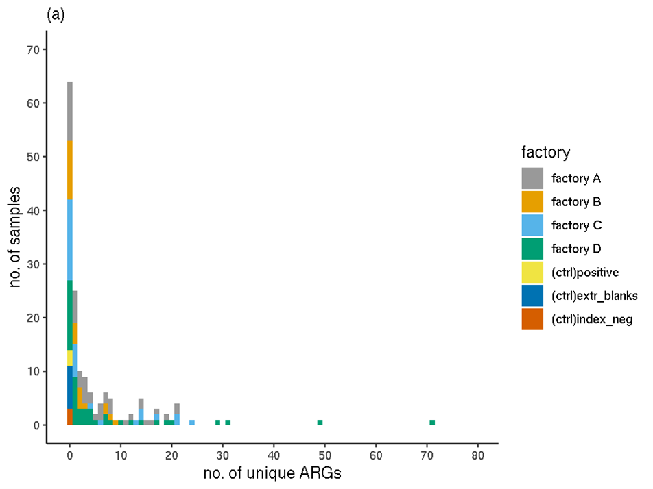
The distributions of the number of unique ARGs in each sample were compared between factories using a Wilcoxon Rank Sum Test (Table 5) with a Bonferroni-Holm adjustment for multiple comparisons. No significant (p<0.05) difference was detected between any pairs of factories. The distribution of ARGs in factories A and B appeared most different but this observation was not significant (p=0.073).

Table 5: Quantiles of the number of ARGs per sample and the significance of differences in distributions between factories

Factory	Number of ARGs per sample - Median	Number of ARGs per sample - 80% Quantile	Significance of difference B	Significance of difference C	Significance of D
A	3	11.2	0.073	0.33	1.00
B	1	2.4	NA	1.00	0.33
C	0.5	13.2	NA	NA	0.37
D	2	10.4	NA	NA	NA

Table 6. ARO drug classes of the 144 unique ARGs which are positive in any sample(s) after the 80%-identity, 80%-coverage filter of the RGI output.

ARO drug class	no. of unique ARGs
aminoglycoside antibiotic	16
carbapenem; cephalosporin; penam	15
diaminopyrimidine antibiotic	10
tetracycline antibiotic	10
fluoroquinolone antibiotic	8
macrolide antibiotic; lincosamide antibiotic; streptogramin antibiotic	7
carbapenem	6
peptide antibiotic	6
phenicol antibiotic	6
fosfomycin	5
glycopeptide antibiotic	5
disinfecting agents and intercalating dyes	3
fluoroquinolone antibiotic; monobactam; carbapenem; cephalosporin; glycylcycline; cephamycin; penam; tetracycline antibiotic; rifamycin antibiotic; phenicol antibiotic; triclosan; penem	3
rifamycin antibiotic	3
cephalosporin; penam	2
fluoroquinolone antibiotic; cephalosporin; glycylcycline; penam; tetracycline antibiotic; rifamycin antibiotic; phenicol antibiotic; triclosan	2
fluoroquinolone antibiotic; tetracycline antibiotic	2
lincosamide antibiotic	2
macrolide antibiotic	2
macrolide antibiotic; aminoglycoside antibiotic; cephalosporin; tetracycline antibiotic; peptide antibiotic; rifamycin antibiotic	2
macrolide antibiotic; fluoroquinolone antibiotic; monobactam; carbapenem; cephalosporin; cephamycin; penam; tetracycline antibiotic; peptide antibiotic; aminocoumarin antibiotic; diaminopyrimidine antibiotic; sulfonamide antibiotic; phenicol antibiotic; penem	2
macrolide antibiotic; lincosamide antibiotic	2
macrolide antibiotic; lincosamide antibiotic; streptogramin antibiotic; tetracycline antibiotic; oxazolidinone antibiotic; phenicol antibiotic; pleuromutilin antibiotic	2
nucleoside antibiotic	2
penam	2
sulfonamide antibiotic	2
acridine dye; disinfecting agents and intercalating dyes	1
aminoglycoside antibiotic; aminocoumarin antibiotic	1
cephalosporin	1
elfamycin antibiotic	1
fluoroquinolone antibiotic; cephalosporin; penam; tetracycline antibiotic; peptide antibiotic; acridine dye; disinfecting agents and intercalating dyes	1
fluoroquinolone antibiotic; diaminopyrimidine antibiotic; phenicol antibiotic	1
fusidic acid	1
macrolide antibiotic; fluoroquinolone antibiotic; aminoglycoside antibiotic; carbapenem; cephalosporin; penam; peptide antibiotic; penem	1
macrolide antibiotic; fluoroquinolone antibiotic; lincosamide antibiotic; carbapenem; cephalosporin; tetracycline antibiotic; rifamycin antibiotic; diaminopyrimidine antibiotic; phenicol antibiotic; penem	1
macrolide antibiotic; fluoroquinolone antibiotic; penam	1
macrolide antibiotic; fluoroquinolone antibiotic; tetracycline antibiotic; phenicol antibiotic	1
macrolide antibiotic; penam	1
monobactam; carbapenem; cephalosporin; penam	1
monobactam; carbapenem; penam	1
monobactam; cephalosporin; penam	1
monobactam; cephalosporin; penam; penem	1
nitroimidazole antibiotic	1

3.4.4.2 Number of samples in which each unique ARG sequence was detected (filtered RGI results)

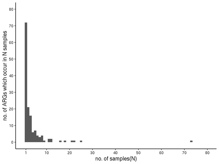
Most ARGs were only seen once. The sequences of almost half of all identified ARGs (71 of the 144) were detected in only a single sample each, coincidentally the same number as the maximum number of ARGs identified in any one sample. Twenty-one occur in two samples, 16 in three, six ARGs occur in four samples. Nineteen ARGs occur in 5 to 9 samples, with 10 occurring in 11 or more (Figure 2). The outlier in 73 samples is rsmA (ARO:3005069) (drug classes: "fluoroquinolone antibiotic; diaminopyrimidine antibiotic; phenicol antibiotic").

Figure 2. Sample-incidence of each ARG (filtered RGI data).

3.4.4.3 ARG incidence (filtered RGI results)

In metagenomic assemblies, the incidence of an ARG in one sample refers to the variety of contexts (assembled contigs/scaffolds) in which it occurs, and not to abundance. For simplicity, the previous summaries of ARG sequences detected in samples was in terms of unique ARGs (defined by unique ARO terms). However, each unique ARG can occur one or more times in each sample; i.e., there can be one or more contig sequences in which the ARG can be detected (indeed, it is possible for a unique ARG sequence to be detected in more than one location within a long contig, in principle). Highly similar, or even identical instances of the same ARG may occur within a sample's set of assembled contigs, for several reasons.

A biological explanation is that the same ARG may occur in the sample in different genomic contexts (i.e. in different positions in the same genome, or in different strains or species, where the flanking DNA may be different).

In theory, with perfect sequencing and assembly, if there were only a single biological context within one sample then all sequencing reads, which sample the ARG and flanking DNA, would be incorporated into a single contig. However, sequencing errors and imperfect assemblies can prevent this.

Therefore, multiple instances of detection of the same ARG sequence in one sample are not uncommon, due to both biological and technical reasons.

 For any sample, the total incidence, in terms of positive contig-ARG matches, is therefore the sum of all of the individual ARG instances. The mean of this incidence sum for all samples for each production plant and for each meat type are shown in Table 7 and Table 8 respectively.

3.4.5 ARG quantification (filtered RGI results)

The sum of a sample's TPM values for all ARGs (ORFs matching ARGs; in this case, fulfilling the 80%-identity, 80%-coverage criteria) represents the total number of biological sequences estimated to be ARGs, out of every million sequences. This includes protein-coding genes, but not other genes (such ribosomal RNA gene variants which confer resistance).

Like the incidence values, the TPM values are indicative. The normalisation applied enables within-sample comparison of abundances, not between-sample, due to the proportional nature of the metric. Therefore, mean TPMs calculated across multiple samples must be treated with caution.

The means of these sample TPM sums are presented in Table 7 and Table 8 for each production plant and each meat type respectively.

Note that when this estimation is performed, all ORFs, of all contigs, are considered, irrespective of whether those ORFs correspond to ARGs, and irrespective of any filtering. Thus, a given ARG in a given sample has the same TPM value in both the unfiltered and filtered results - assuming it passes the filter. However, the total TPM value can be different in filtered versus unfiltered - because in the filtered data, TPMs for ARGs no longer included (due to insufficient sequence identity and/or ARG coverage breadth) will not contribute to the sum.

Table 7. Mean per-sample incidence and mean per-sample estimated quantities, for each production plant.

Factory	Mean incidence of each sample	Mean TPM of each sample
Factory A	5.6	36.86
Factory B	1.9	40.77
Factory C	4.7	21.19
Factory D	7.4	18.00

Table 8. Mean per-sample incidence and mean per-sample estimated quantities, for each meat type.

Meat type	Mean incidence of each sample	Mean TPB of each sample
Chicken	3.5	16.93
Pork	1.6	6.11
Chicken and pork	8.6	21.73
None	7.0	63.12

The all-sample mean TPM values for the 22 ARGs with the highest means (≥0.1) are shown in Table 9.

Table 9. Mean TPM values across all samples, for each unique ARG (filtered RGI results). For brevity, an arbitrary cut-off of TPM = 0.1 has been used, with only those ARGs above the threshold shown.

ARO	Samples	TPM
3005069	rsmA	18.78208
3000816	mtrA	1.17788
3003784	Mycobacterium tuberculosis intrinsic murA conferring resistance to fosfomycin	0.76577
3005009	qacE	0.67982
3004682	aadA27	0.550938
3003836	qacH	0.542619
3002639	APH(3'')-Ib	0.542598
3005098	qacL	0.486602
3005036	BLMT	0.447909
3002884	iri	0.334873
3002660	APH(6)-Id	0.313656
3002950	vanXB	0.29559
3000025	patB	0.243801
3000518	CRP	0.194949
3003369	Escherichia coli EF-Tu mutants conferring resistance to Pulvomycin	0.189135
3000178	tet(K)	0.160697
3002823	ErmH	0.151185
3002554	AAC(6')-Ig	0.150475
3000175	tet(H)	0.136387
3001714	OXA-215	0.122966
3004597	Klebsiella pneumoniae KpnH	0.112272
3000781	adeJ	0.106347

3.4.6 Co-location

ARG co-location was defined as more than one ARG identified on the same contig. Using this metric, a total of 52 (22 for the benchmarking subset), 0 and 24 co-locating ARGs were identified from the Illumina, Nanopore and hybrid assemblies respectively. Full ARG co-location tables for Illumina, Nanopore, and hybrid assemblies are supplied in Appendix 8.

3.4.7 Mobile Genetic Elements (MGEs)

A total of 1,209 contigs from the long-reads assemblies and 11,150 contigs from the short-reads assemblies contained hits to at least 1 MGE. Each sample had at least 1 MGE identified in it. MGE blast results are supplied in Appendix 9.

3.4.8 Metagenomically Assembled Genomes (MAGs)

Of the 15 hybrid assemblies, 3 assemblies contained contigs that were of length 1.5Mb or greater - samples 047, 053 and 087. The single contig from sample 047 was identified as Parvibaculum lavamentivorans.

3.4.9 Taxonomic Identification

Across all samples, a total of 243 genera were identified by Metaphlan3. The most frequently occurring genera were Parvibaculum, Cutibacterium and Methylobacterium, identified in 148, 124 and 119 samples respectively, which were all genera also present in the control samples. When genera which were identified in control samples were removed, 227 genera remained, with the most frequently occurring genera being Rhodococcus, Kocuria and Pseudomonas, identified in 82, 82 and 78 samples respectively. A matrix detailed the identified genera and their relative abundances are supplied in Appendix 9.

3.4.10 Hybrid Assembly Comparison

The benchmarking subset of assemblies were compared, with a focus on the quality of the assemblies. Assembly quality can be roughly estimated through metrics such as the number of contigs (fewer is better), total size of the assembly (larger is often better), contig L50 (smaller is better), contig N50 (larger is better) and the maximum contig size. L50 is defined as the count of the number of contigs whose length makes up half of the assembly/genome. N50 is defined as the sequence length of the shortest contig at half the length of the genome/assembly. The maximum contig size can give an indication of whether an entire genome has been captured in a single contig.

Of note, is the fact that the Nanopore assemblies are often generated from substantially less data than the Illumina assemblies. As such, the assembly size for Nanopore assemblies will be smaller than the hybrid or Illumina assemblies. For this same reason, the number of contigs is also likely be smaller. Additionally, the Nanopore assembler used, Flye, specifies a minimum length requirement, therefore a number of shorter reads will be excluded from the initial assembly steps.

When Illumina and hybrid assemblies alone are compared for number of contigs, L50 and N50, 15/15 hybrid assemblies have fewer contigs, 14/15 have a better L50 and 13/15 have a better N50, suggesting that the addition of longer reads leads to a more contiguous assembly.

3.5 qPCR Results

3.5.1 Quantification of selected AMR genes using qPCR

The qPCR cycle threshold (CT) values for the calibration standards were plotted against the log of the copy number to generate a standard curve. In the samples where target amplification was detected, the CT value was used to derive a measure of the copy numbers by extrapolation from the standard curve.

Quantitative real-time PCR assays exhibit a Limit of Quantification (LOQ) below which CT values are not sufficiently reproducible to reliably estimate the copy number. While we have not formally assessed the LOQ for each of the assays, values calculated at less than 100 copies/µl should be regarded as falling below the LOQ and not reliable estimates of copy number in this study.

These estimates for the copy number values are presented in Appendix 11.

Following the sequencing experiments there was sufficient sample extract remaining in 118 samples to conduct the qPCR analysis. For the 16S gene we obtained valid qPCR results for 117 of the samples, with the calculated copy numbers ranging from 103 to more than 106 copies/µl. For the AMR tet(B) gene we detected only low quantities (less than 100 copies/µl) and in only eleven of the samples. These values for tet(B) should be considered below the LOQ and therefore regarded as qualitative results. With the sul(I) gene, we detected its presence in all the 118 samples tested. In the majority of samples, the values of sul(I) were below the LOQ, but a significant minority of samples showed values above this threshold. To investigate this further we compared the sul(I) copy numbers to those obtained for 16S in the same samples. This is illustrated in Figure 3 below.

Figure 3. Comparison of copy number estimates for the 16S and sul(I) genes. Scatter plot of copy number estimates for each sample with generally increasing trend to higher sul(I) values with increasing 16S copies detected. The marked circle encompasses points where the sul(I) is raised above this general trend.

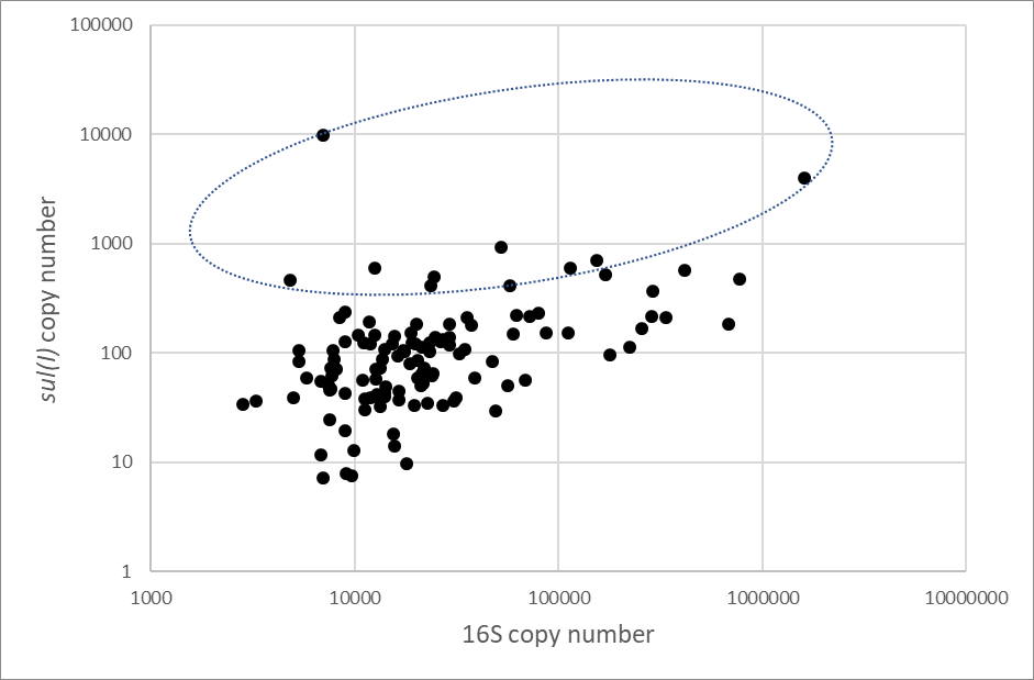
The sul(I) assay used in this study may be amplifying a low level of ‘non-specific’ product which is detected by the SYBRTM Green dye in all biofilm sample extracts (albeit these ‘non-specific’ amplicons produce the expected Tm in the 84.05±0.25C range similarly to genuine sul(I) amplicons). This would suggest that in the majority of samples the sul(I) detections are not genuine and are more reflective of the quantity of bacteria in the biofilm sample. There are, however, a number of sample where the sul(I) detections are raised above this background level and which are more likely to have resulted from genuine detections. We would estimate that there are 8-10 samples where the sul(I) detection is more likely to be genuine.

3.5.2 Normalisation and comparison to metagenomic data

As stated in section 3.4.5, TPM values represent proportions of each gene or DNA fragment among all of those sequenced. Ultimately this is because the DNA sequence data is compositional and does not provide information on absolute quantities.

We therefore attempted to use the qPCR results for the two specific ARGs tet(B) and sul(I), and the general bacterial qPCR (16S rRNA gene), as external references to calibrate the TPM values for each of the samples for which qPCR data was available. We also incorporated the ORF sequences which in silico PCR (ecoPCR software) had indicated to be tet(B) or sul(I). These would not necessarily all have been found by the RGI/CARD analysis, especially after we had applied the strict filter to these results. We confirmed that sequences corresponding exactly to the primer pairs used for tet(B) and sul(I) are present in the CARD database. Each pair is present in one reference sequence, which have the expected gene annotations.

Additionally, as 16S data was available for all of the samples assayed by qPCR, and we had calculated TPM values for all of the in silico PCR 16S sequences, we used these data to calibrate the total-ARG TPM values for these 117 samples. The numbers of samples positive by each method is shown in Table 10.

Table 10 Numbers of samples positive for each gene by sequence analysis and qPCR. 16S refers to the sequences amplified by the 515-806 primers used in this study and not to specific variants which are in the CARD database.

Sample	unfiltered RGI	filtered RGI	ecoPCR	qPCR	qPCR, est ≥ 500 copies/μl
tet(B)	19	0	1	11	0
sul(I)	40	7	11	117	9
16S	N/A	N/A	144	117	117

3.5.2.1 tet(B)

Prior to filtering, the tet(B) RGI results showed a small number of samples being positive; however, all of them had very poor coverage of the reference sequence and did not pass the filter. The single ecoPCR in silico amplicon sequence was checked against the NCBI nt database, but no similarity to a known sequence was found. This indicates that this sequence is probably in a misassembled region of a metagenomic contig, flanked by matching primer sequences. The metagenomes are therefore negative for genuine tet(B) sequences, which is largely consistent with the qPCR results. We therefore did not consider tet(B) further.

3.5.2.2 sul(I) in relation to 16S

Similar numbers of samples were positive for sul(I) in the filtered RGI and ecoPCR results (Table 10). The 7 filtered RGI-positive are a subset of the 11 ecoPCR-positive. We confirmed that the other 4 were all RGI-positive before filtering. Each of the 11 had one in silico amplicon and we examined these to confirm that they are highly similar to the expected sequence. qPCR analysis had been applied to three of these 11 samples. The positive samples and their metagenome-estimated sul(I) relative abundances (TPM values) and copy numbers estimated from qPCR are shown in Table 11. This also shows the TPM values calculated for all of the ecoPCR 16S sequences, and the qPCR-estimated 16S copy numbers for those samples which were assayed.

Table 11. In silico positive ORFs and abundances, and qPCR abundances of sul(I) and 16S for the 11 samples positive for a predicted sul(I) amplicon. Cells marked with a dash indicate samples which were not assayed with qPCR.

sample ID	sul(I): filtered RGI ORFs	sul(I): ecoPCR ORFs	sul(I): rel. abund. (TPM)	sul(I): est. copy no.	16S: rel. abund. (TPM)	16S: rel. abund. (TPM) sul(I): copy no/TPM	sul(I): copy no/TPM	16S: copy no/TPM
053	1	1	0.05	-	317.80	-	-	-
078	0	1	0.05	-	455.43	-	-	-
079	1	1	0.51	-	600.71	-	-	-
080	0	1	0.15	4,034	604.50	1,607.670	26.944.9	2,659.5
083	1	1	6.12	-	660.79	-	-	-
084	1	1	0.63	-	667.76	-	-	-
085	1	1	1.68	-	567.77	-	-	-
088	1	1	0.18	-	520.67	-	-	-
101	1	1	0.29	601	298.37	113,579	2,038.4	380.7
137	0	1	0.26	-	258.21	-	-	-
223	0	1	0.32	412	104.53	23,647	1,275.2	226.2

In principle for any gene, the ratio of the copy number (absolute, per μl) to the TPM (relative abundance) represents a scale factor to convert the TPM values to copy number equivalents. This is expected to vary considerably between samples, because the absolute amounts of DNA in the original samples may differ considerably. This ratio is shown in Table 11 for the three samples with qPCR data. If all of the sequencing data, TPM estimates and qPCR copy numbers are consistent, then this scale factor should be the same for all genes. However, the same ratios for 16S differ from the sul(I) in all three samples, by a factor of 5 to 10.

This indicates that if the qPCR data is indicative of the true abundances, the metagenomic sequencing and/or abundance calculations are not sampling these two genes proportionally. Although two of the samples' sul(I) copy numbers are close to the limit considered to give reliable estimates (one is below it), the third (sample 080) has the second highest sul(I) copy number in any sample. This sample had a high number of metagenome sequencing reads (123 million following contaminant removal).

3.5.2.3 Total ARGs in relation to 16S

We used the same approach as in the previous section, to estimate copy number equivalents for all protein-coding ARGs collectively. This could be done for all samples to which qPCR had been applied for the 16S gene, and thus had a copy number:TPM ratio available for 16S. The same principle was applied as for the sul(I) gene, but here the sum of all ARG TPMs was used for each sample, rather than the TPM of a single gene. This was obtained by summing the KALLISTO-output TPMs for all ORFs which featured a positive RGI prediction which passed our identity/coverage filter. Multiplying this sum by the 16S copy number:TPM ratio thus applies a sample-specific scaling. In theory, the result is a copy-number equivalent measure for the set of any/all ARGs, collectively, which can be compared between samples. This relies on the assumption that the ratio would be generally similar for these ARG genes as for 16S, which was found not to hold for sul(I), albeit with very few data points available (previous section). The results of this normalisation should therefore be treated as indicative only. For the 118 samples involved, the results are shown in Appendix 11.

In summary:
scale factor = 16S copy no. /  TPM  (1)
normalised total ARG abundance = scale factor x total ARG TPM (2)

Figure 4 shows that the relationship (1) between 16S copy number from qPCR, and the 16S TPM values appear not to be random. There are no samples with high copy number estimates and low TPM. Nonetheless, as expected there is considerable variation in the ratio (used for the normalisation), particularly to TPM values greater than around 200.

Figure 4. Abundances of 16S gene in samples which were assayed by qPCR. Copy numbers (copy no/ μl) were obtained from qPCR. Relative abundances were calculated from metagenomic sequencing. 

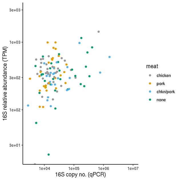
The unnormalised relative abundance values (TPM) should in principle not be compared between samples if absolute comparisons are of interest. One comparison of interest is therefore the normalised (2) values versus the unnormalised TPM (Figure 5). This shows that for this data set, there is a reasonable correlation between the two.

Figure 5. Comparison of estimated total-ARG copy numbers and total ARG relative abundances for each sample. The copy numbers were obtained by normalising the relative abundances by a sample-specific scale factor obtained from the 16S abundance analysis.

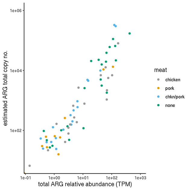
Figure 6 shows a comparison of the unnormalised TPM abundance values and the normalised abundances, for samples categorised by factory. Figure 7 Figure 7 shows the same for samples by meat type.

Figure 6. Total ARG abundances for each factory. (a) Unnormalised relative abundances. (b) Normalised abundances (estimated copy numbers per μl).

 

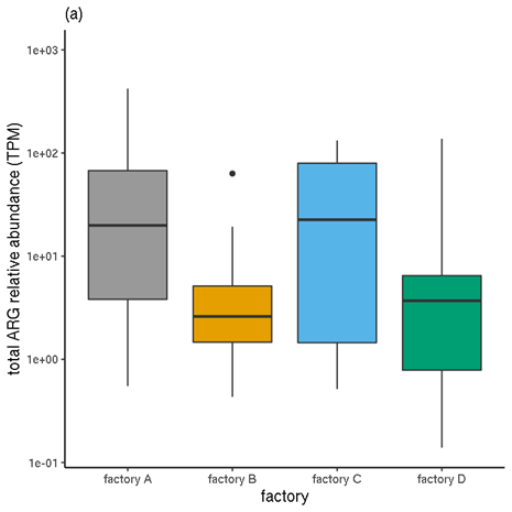
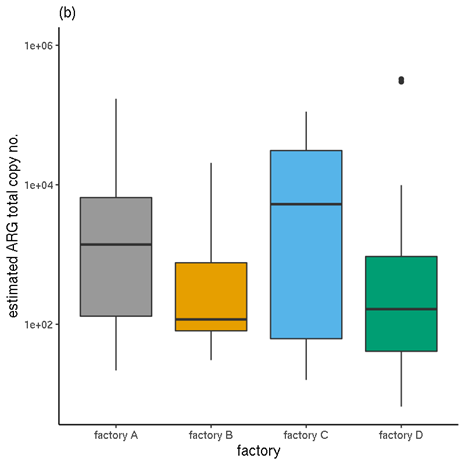
3.6 AMR burden from the UK diet and the possible link to biofilms

In this section, we consider the implications for UK dietary sources of ARGs. Existing information on AMR detected in retail meat samples is first summarised, for comparison. 

Collection of the biofilms samples was designed to be representative of the UK diet as far as possible. However, there were some practical constraints, so we include a discussion of the total UK consumption of the relevant meat types and what this means for the representativeness of the sampled biofilms.

3.6.1 AMR phenotype of E. coli isolates data from EU harmonised surveys

The focus here is on the most recent UK data compiled by the FSA. Sampling was designed to represent 80% of the retail market share and 80% population coverage. In the most recent UK survey at least 300 samples were collected for each of 3 retail meat categories (beef, pork, poultry). Summary tables are presented below for fresh retail samples of UK Beef (Table 12), Pork (Table 13) and Chicken (Table 14) collected between 2015 and 2019. The type of samples collected varied between years. The proportion of positive samples is much higher for chicken than for other meat types.

Table 12. Summary of UK Beef samples 2015-2019 from the EU harmonised surveys

Year (UK data)	Total beef samples	ESBL CTX	AmpC	ESBL CTX + AmpC
2015	312	1	1	0
2017	314	1	1	0
2019	289	1	0	0

Table 13. Summary of UK Pork samples 2015-2019 from the EU harmonised surveys

Year (UK data)	Total pork samples	ESBL CTX	AmpC	ESBL CTX + AmpC
2015	312	1	1	0
2017	310	0	1	0
2019	285	2	1	0

Table 14. Summary of UK Chicken samples 2015-2019 from the EU harmonised surveys

Year (UK data)	Total chicken samples	ESBL CTX	AmpC	ESBL CTX + AmpC
2016	313	75	49	2
2018	309	23	16	3

Some additional information is provided by the reports linked in Section 2.8 that may be relevant. For example, in 2019 none of the isolates obtained from UK samples were carpabenamese-resistant or colistin-resistant (mcr-1, mcr-2, mcr-3 are the mobile colistin resistant genes tested for). Also, although 315 beef and 313 UK pork samples were collected in 2019, not all were suitable for reporting due to technical issues. In 2018, of the 309 chicken samples the type of chicken samples was listed, and these comprised 125 whole chicken, 112 chicken breasts and 72 other cuts, e.g. quarters, legs, thighs drumsticks. It was noted that the proportion of positive samples was higher for skin-off chicken, which may suggest the potential for cross contamination during the skin removal process. None of the isolates obtained from these samples were resistant to carbapenem or mcr-1, -2, or -3. Processed pre-prepared chicken including goujons, ready meals, marinated, breaded, battered, frozen or cooked chicken, were all excluded. The AMR samples collected in the current project, and the consumption survey data, do include these value-added poultry products, so there is a mismatch in the type of products when trying to link with the harmonised survey data. Additional contamination, or reductions in contamination, that may arise from these processes are therefore not represented in these data. 

Table 15 lists those gene classes consistent with E. coli that were found in the biofilm samples, and/or those that were found in the survey of retail meat. There were 12 gene classes found in the biofilms samples but not recorded in the meat survey results.

Table 15. Gene classes found in biofilms samples, meat survey, or both, that are consistent with E. coli and were predicted to confer antibiotic resistance

Found in meat survey but not biofilms	Found in biofilms samples but not meat survey	Found in biofilms samples and meat survey
polymyxin antibiotic	disinfecting agents and intercalating dyes,  nitroimidazole antibiotic,  elfamycin antibiotic,  peptide antibiotic,  penem,  nucleoside antibiotic,  monobactam,  rifamycin antibiotic,  triclosan,  fosfomycin,  glycopeptide antibiotic,  acridine dye,  aminocoumarin antibiotic	aminoglycoside antibiotic, macrolide antibiotic, fluoroquinolone antibiotic, penam, carbapenem, cephalosporin, sulfonamide antibiotic, glycylcycline, cephamycin, tetracycline antibiotic, phenicol antibiotic, diaminopyrimidine antibiotic

3.6.2 ARG detection in retail samples of chicken

In a scoping study of ARGs measured in retail chicken samples from the UK and Ireland [38] 76 samples were collected in total, including thigh (30), leg (27) and breast (19) meat portions. In Table 5 of McNeece et al (2014) the numbers of samples found to be positive for selected ARGs are listed. The ARGs found were: sul3 (6), tetD (12), tetE (18), cmlA1 (7), fox (44), catB8 (4) and cmy (62). The study used a statistical test to assess whether there was a difference in prevalence between each pair within the 3 source groups (UK-free range, IE-intensive, UK-intensive). Testing for bacteria was also reported in this paper, using Denaturing Gradient Gel Electrophoresis (DGGE) followed by sequencing of the products to identify some of the Gram-negative bacteria present. However, it was noted in the discussion that linking specific resistances to species is something that requires further work. 

3.6.3 Consumption of Beef, Pork and Chicken products summarised from UK NDNS surveys

Trends in UK meat consumption (2008/9 – 2018/19) are addressed in Stewart et al. (2021) [42]. Within most population sub-groups, a reduction in overall meat consumption per day was inferred from the survey data. A statistically significant negative trend was reported for red meat, particularly for beef and sausages, but not in pork nor in burgers. For the current project, we attempted to reanalyse the UK consumption levels to extract information about specific relevant food types to answer questions about the UK burden from AMR in processed meat.

Table 16 shows the proportions of individuals within different subpopulations consuming the meat types of interest (beef, pork and poultry) after accounting for disaggregation into raw ingredients, summarised from the NDNS data. Minced beef, corned beef and cooked chicken slices are included as these make up significant proportions of the consumed items. Corned beef and wafer-thin chicken slices are types of ready-to-eat products, so the burden from these products is not considered here. Similarly, the consumption of pork will include a contribution from ready-to-eat ham. The burden from these and other ready-to-eat products was considered in a separate FSA project FS301050 [43].

Table 16. Proportion of individuals consuming one or more of the food types (Beef, Pork, Chicken)

Population	Beef Total	Beef Mince	Beef Corned	Pork Total	Poultry* Total	Poultry* Wafer-thin chicken slices
Adults (18-64)	62.8%	41.3%	4.2%	78.9%	88.2%	6.2%
Older adults (65+)	64.8%	37.3%	8.4%	82%	85.2%	4.9%
Children (0-10)	60.2%	48.9%	2.4%	70.5%	87.7%	18.2%
Children (11-17)	63.3%	47.3%	2.5%	82.1%	92.2%	11.6%
All	62.1%	44.4%	3.7%	76.5%	88.3%	11.6%

*The NDNS category is poultry and includes turkey consumptions

Plotting the amount of individual meat types as a function of the survey year also allowed us to investigate individual trends in products. Overall, we found that poultry is consumed by a larger proportion of the population than the other meat types, although pork is a close second. There is evidence of a general reduction in amounts of beef and pork consumed in recent years, but the average daily amounts of chicken consumption do not show a substantial change over the 11 years of the NDNS survey. The same conclusion was reported in Stewart et al (2021) where poultry and game birds were included as ‘white meat’ and found not to have changed significantly.

The individual meat types reported were also investigated, to help determine whether the collected biofilms samples were representative of current UK consumptions. We found that:

• Food names used to describe beef are: Steak, minced, topside, roast, cooked slices, ox tail, ox tongue, pastrami. Beef burgers did not appear in the summaries because these were classified using the raw ingredients (beef mince stewed) in the recipes database.
• Food names used to describe the types of pork consumed after recipe disaggregation are: Bacon (smoked, middle, back), Pork crackling, Pork shoulder, loin, belly, chops, tongue, ribs, Diced, Minced, Ham (smoked and unsmoked), Parma ham, Brawn, Polony, Haslet, Salami, Gammon, Roast pork roll/slices.
• The types of chicken described in the survey are: Chicken breast, roast, boiled, casserole, barbecued, slices, leg/drumsticks, wing, roll.
• The types of turkey consumed (although with far fewer consumers) are: Turkey breast, roast, slices, mince, roll/slices.

In summarising the proportion of individuals that are consumers within a (sub-) population, we have included wafer thin chicken slices as this is the only meat processing type that has a substantial number of consumers. We also note that this proportion is higher in children than in adults.  As explained below, this does not necessarily represent chicken slices purchased as ready-to-eat chicken. Rather, it may be an artefact from using the recipes database because ‘wafer thin chicken slices’ appears there as a component of processed chicken products such as chicken burgers.

The summaries presented above relate to overall meat consumptions from broad classifications (beef, pork, poultry) and include ready to eat cooked foods and disaggregated ingredients from recipe dishes or from raw meat ingredients that cannot be linked to individual processed meat products directly. Even where a component food type might appear to represent a consumed product, they may also appear as part of a different product type. For example, there are recipes for chicken burger that include ‘chicken slices wafer thin not smoked’, so the chicken from the chicken burger is represented as wafer thin chicken slices. Other chicken burger recipes include ‘chicken cass light and dark meat only’ (sic). Coated chicken pieces takeaway is defined as ‘chicken boiled light meat only’. The translation from meat product to the raw primary meat types often leads to very different interpretations and makes it impossible to link the results directly to the processed meat samples. Another way to summarise the survey data that avoids these difficulties is to consider the product level descriptions without using the recipes. This was considered to be more useful for assessing the types of products purchased by consumers, and therefore the representativeness of the products sampled from the meat processing plants. 

The NDNS was therefore re-examined to assess consumption by product type. The overall meat-related product categories in the NDNS are: Bacon and ham, Beef veal and dishes, Lamb and dishes, Pork and dishes, Chicken and turkey dishes, Coated chicken, Meat pies and pastries, Other meat and meat products, Sausages, Liver and dishes, Burgers and Kebabs. The numbers of consumers and some key individual products are shown in Table 17. These values give an indication of the relative numbers of individuals (from the total surveyed 18338) consuming particular food types. In principle, linking consumption of individual products to ARG levels in those products may provide information about the relative potential burden of AMR from biofilms linked to processing for those food types.

Table 17. Summaries of meat product consumptions recorded in the NDNS rolling program years 1-11 (2008/9-2018/19) combined with the DNSIYC for infants. The product groups are ordered by the total number of consumers. The total number of individuals in the data is 18338. Italicised food items are considered as ready to eat foods so are not in scope for the project. The bold food types are those processed in the sampled plants

Meat product group	Number of consumers	Mean daily consumption (g) for consumers only	Main food types (by number of consumers)
Chicken and turkey dishes	11863	92.9	Chicken breast grilled (4051), Chicken roast (3830), Chicken boiled (2058), Wafer thin chicken slices (729)
Bacon and ham	9831	42	Ham, not smoked (6618) Bacon rashers grilled (3975) Bacon rashers fried (1151)
Beef veal and dishes	8504	79.5	Beef mince stewed (4039), Stewing steak stewed (954), Beef topside roast (938)
Sausages	6753	57.9	Pork sausages, grilled (4213), Frankfurter (593), Premium pork sausages (529), Chorizo (360)
Coated chicken	4274	68.7	Chicken goujons (1178). Coated chicken pieces takeaway (1092), Chicken breast coated grilled (470), Chicken burger takeaway (337)
Meat pies and pastries	3540	69.1	Sausage roll (1456), Chicken pie frozen (345), Cornish pasty (199), Pork pie buffet (147)
Pork and dishes	3149	62.6	Pork loin chops grilled (939), Pork loin joint roasted (512), Diced pork stewed (279), Pork & beef meatballs (230)
Burgers and kebabs	2372	62.4	Beefburger 100% grilled (673), Beefburger economy grilled (441),  Cheeseburger takeaway not ¼ pounder (402)
Other meat and meat products	2276	43.1	Salami (451), Corned beef not canned (363), Peperami (258), Corned beef (210), Black pudding fried (152)
Lamb and dishes	2237	74.7	Lamb leg roast (440), Lamb mince stewed (308), Lamb loin chops grilled (287), Lamb scrag and neck stewed (270)
Liver and dishes	539	36.1	Liver pate plastic wrapped (225), Lambs liver (88), Liver pate deli (58)

3.6.4 Representativeness of the sampled factory areas for consumed food types

The meat processing factories include areas that process multiple product types, and so there is not a simple one-to-one relationship between biofilms and single food types. However, roughly classified meat types and numbers of samples associated with their processing can be listed as follows:

Factory A: added value chicken (4), brine (4), chicken + brine (3), chicken breast (11), diced chicken/fillets/portions (7), whole bird (3)

Factory B: pork (8), bacon (3), Wiltshire brine (2)

Factory C: pork (17), chicken (2), all meats: pork/chicken/beef (3)

Factory D: pork (5), chicken/chicken products (5), chicken and pork (25), chicken and pork sausages (6), chicken burgers/mince + pork burgers (2) 

Food type descriptions included in the sample metadata and in the NDNS consumption diaries food are sometimes ambiguous and do not use a common coding system. There is some uncertainty therefore about the relative amounts of individual products processed. However, by comparing these terms against those products most commonly consumed in the survey (Table 17) it is possible to identify any missing food types. Beef mince products seem to be the most commonly consumed processed meat types that are not well represented in the processing types of our sampled factories. Other highly consumed meat products do seem to be represented, especially for the important category of chicken products, but also pork sausages and bacon. In some cases, there are highly consumed food product categories that are not described in sufficient detail to be able to determine whether they can be linked to one of our meat processing plant biofilm samples. The main examples seen in Table 17 are ‘chicken roast’ and ‘chicken boiled’.

3.6.5 Assessing population burden due to processing

If individual ARGs are identified and can be linked to one or more food types based on the classifications and summaries outlined above, then a simple process could be followed to estimate the proportion of individuals consuming those food types and therefore the proportion of individuals exposed to specific ARGs. This could be extended to consider the burden from broader general food types represented in the data (e.g. burden from chicken or burden from pork products). This general approach was used to estimate the measure of burden in the ready-to-eat food project FS301050. There are several limitations to this approach that mean it is a highly uncertain – and potentially misleading – estimate of the true overall burden. Within the current project it was therefore agreed that such an estimate would not be derived. Details of the uncertainties and suggestions for dealing with these are summarised in Section 4.2.7.

3.6.6 Comparing ARG prevalence in samples taken from chicken lines to ARG prevalence in bacteria detected in chicken

The proportion of national chicken samples which contained each of 47 ARGs [38] were compared with the proportion of biofilm samples in each factory that contained the same ARGs. Estimates of how much larger or smaller the factory biofilm proportion was compared with the national chicken proportion are shown in Figure 8 and Table 18. Of the 47 ARGs tested for on the array used for the chicken samples, five ARGs were detected in factory biofilms containing sequences consistent with Gram-negative bacteria: AAC(3)-Ia, cmlA1, sul1, sul2, tetE. Seven ARGs were detected in UK chicken samples catB8, cmlA1, cmy, fox, sul3, tetD, tetE.  Although three ARGs were detected in factory samples that were not detected in chicken samples, the prevalence was low enough for the difference in proportions to be not significant (i.e. the underlying proportion in the population of chicken portions might be the same as the underlying proportion of biofilms). Cmy, fox and tetE were not detected in factories and were detected at prevalences that were significantly higher in UK chicken (again assuming that the prevalences are comparable). This analysis just shows that we didn't see that ARGs at high prevalences in biofilms were not present in similarly high proportions of chicken samples.

Figure 8: difference in prevalence of AMR in biofilm samples that contain Gram-negative bacteria and intensive UK chicken samples

 

 

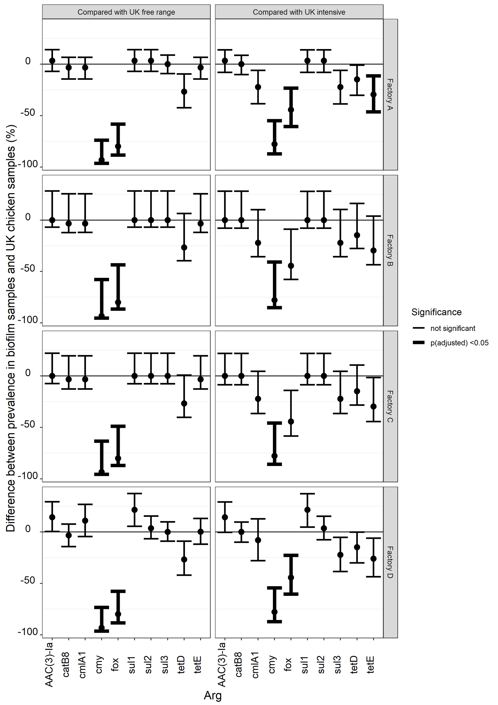
4.1 ARG Findings

After filtering by length and identity, 144 ARGs were detected in the full set of samples, and none occurred in any controls. Of the 144 biofilm samples that were successfully sequenced, 96 samples were positive for at least one ARG. In this context, when we refer to an ARG, it may more properly be thought of as a gene that could potentially be associated with antimicrobial resistance (see section  4.2.3). Specifically, the definition of an ARG in this project includes any gene that is annotated as an ARG in CARD reference database.

When we consider the distribution of ARG frequencies (i.e. how many different ARGs are found in samples from each plant) these do appear similar. No plant has a clearly higher or different ARG frequency distribution, although Factory B has a lower (though non-significant) median number of ARGs per sample than Factory A (p=0.07). There is also an apparently longer tail for samples from factory D – the four most ARG-heavy samples were from this factory. Furthermore, as well as having the four samples with the highest number of different ARGs in them, factory D also had the highest average incidence of the ARGs across its samples. This means that, overall, each ARG found in plant A was found more often within a sample than were ARGs in other plants. This could be due to the same ARGs being found in multiple different bacteria or mobile genetic elements within a sample, for example.

The picture is similar with the different meat types processed, with samples associated with “pork and chicken” (that is, plants or lines through which both pork and chicken are processed) having a similar distribution to samples from factory A. However, it is difficult or impossible to disentangle the effect of meat type from the effect of factory, due to the small number of factories, with most focussing on only one or two meat species. Interestingly, there is some indication that the processing machinery exposed to non-meat media, i.e. brine or dextrose water, have relatively high incidence, although low sample numbers for these sample types make it impossible to draw firm conclusions. Both dextrose water samples had non-zero ARG counts, as did five of the six brine samples, compared with 88 of the remaining 136 other samples. There is some evidence to suggest that the presence of dextrose can enhance biofilm formation [44]. 

Regarding taxonomic assignment, although some of the formal ARG names in the ontology include names of bacteria, others may occur in multiple species. An analysis of the taxonomic origins of the ARGs is beyond the scope of this report, and further analysis is of interest to determine any implications of the above results for the types of bacteria found (for example, halophiles).

Of the ARGs detected, rsmA was found in by far the highest number of samples (n=73), and had the highest mean TPM value across samples, suggesting that where it is found it constitutes a relatively high proportion of all ARG reads within a sample. rsmA regulates virulence in Pseudomonas aeruginosa [45], and rsmA homologs (csrA) can regulate a wide range of factors including biofilm formation [46]. rsmA is annotated as an ARG in this instance as it can also be involved with regulation of multidrug efflux pumps, with an rsmA mutant showing increased resistance to amikacin, nalidixic acid, trimethoprim, ceftazidime and gentamicin, and decreased resistance to polymyxin B and colistin [47]. The widespread detection of a P. aeruginosa-associated gene is not surprising, as P. aeruginosa is known to be able to form biofilms on surfaces commonly used in food processing environments, including various plastics [48, 49] and stainless steel [49].

Other ARGs of note with high mean TPM values include the qac genes qacE [50], cqaH [51] and qacL. These genes encode small multidrug resistance (SMR) efflux pump genes carried on plasmids and transposons, which can confer resistance to quaternary ammonium compound (QAC) biocides [52]. QACs are widely used in industry as biocides, and biofilms have been demonstrated to increase resistance to QACs [53], so it is again unsurprising that qac genes are identified in biofilms in meat processing plants. While these genes can potentially confer resistance to QACs, they do not appear to confer resistance to antibiotics. However, they could still be of interest as they may promote the transfer of antibiotic resistance genes within the microbiome [54] and may mean that bacteria are more likely to survive and persist in biofilms if they are resistant to the use of QACs.

Some of the other ARGs identified highlight the difficulties associated with metagenomic sequencing. ARGs annotated as belonging to M. tuberculosis (Mycobacterium tuberculosis intrinsic murA conferring resistance to fosfomycin) and K. pneumoniae (Klebsiella pneumoniae KpnH) are unlikely to be associated with the taxa in question. Given the 80/80 percent identity/length these hits could well be to homologs of these genes in related taxa (for example, K. oxytoca) or even more distantly related species. This caveat is also relevant to the observations of P. aeruginosa rsmA discussed above, as upon further inspection, several of the identified ARGs appear to share a high percentage identity to csrA, and could therefore potentially be present in non-Pseudomonas species.

Other ARGs found at high mean TPMs illustrate the complex nature of other aspects of the analysis of biofilms undertaken in this project. Genes potentially involved in resistance to tetracycline (tet(H) and tet(K)) were found at relatively high mean TPMs, which does to some extent justify the selection of a tetracyline resistance gene as one of the qPCR targets. The specific gene chosen, tet(B), was not among the highest TPM ARGs, and neither was sul1, but the timescales of the project required that qPCR targets were identified ahead of the results of the sequence analysis being available. In this case, the results of FS301050 were used to select genes identified in cooked meats. 

There are important difficulties in drawing firm conclusions about the ARG burden of biofilms, for example, the degree to which they contribute to the ARGs present on foods produced in biofilm-containing factories. This is principally due to lack of comparable samples. There is little published in the literature that applies the same techniques used here to relevant sample types (for example, secondary meat products), and no samples were taken in this project from intake carcasses/outflow products. That being the case, we have taken two published studies, using two different approaches, and attempted to compare our data to them.

One study is a small-scale study of ARG prevalence in chicken processed in the UK and Ireland [38]. In that study an array-based detection method was applied, which was deemed a relevant comparison as it was a molecular method, not targeting a single bacterial species, although in this instance it did follow an enrichment for Gram-negative bacteria. That being the case, we also confined our comparisons to biofilm samples which contained evidence of Gram-negative bacteria. Other limitations to the comparison included the limited number of ARGs tested for, the small number of samples tested by the array, and the fact that the samples were not contemporaneous with the biofilm samples. Overall observations of ARGs were observed in a smaller proportion of Gram-negative samples taken from biofilms than were seen in Gram-negative samples taken from chicken.  There may be a number of different drivers for this observation. One possibility is that bacteria in factory biofilms actually contain fewer ARGs than bacteria in chicken. Another reason for this observation may be that the method used to test for ARGs in chicken, is more sensitive than the method of detection applied to factory biofilm. Hence, it is difficult to tell whether looking for ARGs in chicken may be more informative than looking for ARGs in biofilms, or whether looking for ARGs using the method applied to chicken samples is more informative than looking for ARGs using the method applied to biofilm samples.

Even more difficulties are encountered when trying to compare our data with phenotypic results from isolates from retail meat surveys. In predicting which genes confer resistance to antibiotics and comparing the biofilms with retail meat surveys (Section 3.6.1) some simplifications were necessary. A major caveat is that the particular genes identified in our study do not necessarily confer resistance to all antibiotics within a particular class. However, the antibiotic class was the only annotation available from CARD/aro and it was therefore relatively simple to identify common classes. A more detailed investigation to check for resistance to individual antibiotics would involve a specific literature search and would be a much larger task, because all 26 antibiotic drug classes (Table 15) would need to be checked.

An assessment was also made to identify which of the genes found in our study are consistent with E. coli, though some of these genes may also be present (with exactly the same sequences) in other species. Multiple resistance mechanisms are observed, with some conferring resistance by their presence (as single gene system) and others as efflux pumps or parts of operon. Those that are not single gene systems do not necessarily imply phenotypic resistance, so it may be that they should be excluded form analysis. For example, the following ARGs were found in our biofilm data and are not single gene systems (number of samples shown in parentheses):

CRP (12), emrR (12), msbA (9), Klebsiella pneumoniae KpnH (8), marA (5), baeR (1), Escherichia coli marR mutant conferring antibiotic resistance (1), Escherichia coli soxR with mutation conferring antibiotic resistance (1), Escherichia coli soxS with mutation conferring antibiotic resistance (1), PmrF (1), Klebsiella pneumoniae KpnF (1).

The assessment could be repeated with these genes excluded. This kind of assessment is feasible when small numbers of metagenomically-identified ARGs are concerned, but less so for large scale studies.

4.2 Technical Considerations

4.2.1 Sampling Strategy

The sampling of biofilms was limited to only a small number of factories. However, as shown in Section 3.6.3, and particularly summarised in Table 17, the main types of secondary meat products consumed within the UK are represented by processing within these factories (chicken products, pork sausages and bacon). Furthermore, in Section 3.6.4 the representativeness of the sampled production areas within these factories was considered, comparing the types of meat processed there with the main consumed types. We believe that the samples provide a good coverage of the most commonly consumed items. The only category that is less well represented is minced beef or beef burgers. 

Data were not available to quantify the amounts of processed meat purchased from these factories as a proportion of the total UK purchase and consumption. As a result, only limited information is available about the between-factory variation in ARGs. A quantitative estimate of the proportion of consumers represented by the survey would require information about all processors within the meat supply chain.

With regards to the actual sampling implementation, due to covid restrictions we were unable to be physically present for any of the sampling locations or times. We were reliant on the goodwill and expertise of the factory staff to take samples, for which we are very grateful. However, this does introduce another source of variability.

4.2.2 SOP Development

After recommendation by experts in food production hygiene, the use of the Biofinder spray was trialled for identifying biofilms. However, as the Biofinder spray contains hydrogen peroxide, there was a concern that it may degrade any DNA present prior to sequencing. After sequencing the test material, the Biofinder + MGW rinse and the non-Biofinder treatments generated similar percentages of both bacteria present. The non-Biofinder method detected more Pseudomonas, though all methods detected comparatively little Pseudomonas. This was interesting as twice as much Pseudomonas was inoculated onto the slides as E. coli. The reasons for this are unclear. Potentially the E. coli was able to replicate faster than the Pseudomonas from the same initial inoculum, as has been shown previously [55], or was able to form a stronger biofilm by attaching and proliferating more readily. Unfortunately, a detailed investigation of this was beyond the scope and budget of the current project. 

4.2.3 Sequencing considerations

Challenges which affected some samples were low DNA yields, and possible contamination.

The factories reported that Biofinder foaming was not frequent, and so factories were required to sample even where it did not foam, but in places where we anticipated likely biofilm formation. Even where Biofinder was negative, samples corresponded to the definition of biofilms used in this report for example, bacteria and other microorganisms that remain adhered to a surface (presumably by extracellular secreted substances) immediately after surface rinsing. However, this potentially would have led to some of the lower DNA yields. Although only two samples generated unusably small numbers of DNA sequence reads, sampling from heavier biofilms (if present) may have generated higher DNA yields overall.

Regarding the source of contamination, the sampling protocol was shown to work with the test biofilms, which suggests that factories did not generally harbour strong biofilms, at least in the samples tested. However, there was a significant amount of DNA sequence obtained in the controls. This is itself is not surprising, as the volume of control samples   incorporated into the sequencing pool is the same as the average volume pooled across all samples. Given the high depth of sequencing undertaken in this research project, even relatively low amounts of DNA obtained from the controls would be expected to generate sequence data. Nevertheless, the amounts of sequence generated for some of these controls is very high. This suggests at least two phenomena – the relatively low yields of DNA found in general among the biofilm samples, and the presence of contaminant ‘kitome’ DNA in the sampling and/or DNA extraction kits.

Increased depth of sequencing compared to previous studies (FS301050) improved our ability to assemble the DNA reads into contigs and meant that we could use assemblies rather than short reads. However, the type of sample also assisted in this regard (the previous study involved obtaining bacterial DNA from the surface of or within host organisms, increasing problems of non-bacterial contamination). It might also be expected that the bacterial populations of the biofilms are less diverse, generally providing greater coverage for any given genome segment.

This is beneficial because we are more likely to obtain longer and more accurate hits to ARGs which extend beyond the 250bp length of a single read. It also allows us to capture regions which may be unique to particular taxon, thus taxonomic identification of ARGs could be easier and more accurate. Furthermore, we benefit from error checks that happen during the assembly process, so have more confidence in the contigs produced. The potential disadvantage of analysing assemblies is that some genes/fragments represented by very few reads would not be incorporated into any contigs, effectively giving a false negative. This may affect samples with particularly low read counts. With short-read analysis, we previously showed that it is possible identify some individual reads as almost certainly originating from a longer ARG fragment (FS301050). However, in the general case, analysis of unassembled short reads presents far greater complications in filtering out false positives, and therefore our view is that ARG sequence detection is better performed on assemblies.

Long-read sequencing appeared to perform better than in previous studies (FS301050), which is perhaps surprising due to the generally low amounts of DNA obtained in this study. This may reflect advances in ONT library preparation and sequencing chemistry. The average read length was still slightly lower than the 1-2 kb which would be ideal for the assembly software (Flye). However, hybrid-assembly with the Illumina short reads was very successful, though not in every case were the N50 and L50 scores better than those in the Illumina-only counterparts.

It is more likely that we would obtain structurally accurate contigs with hybrid assemblies, providing more accurate co-location information, in addition to assessing the possible impact of any MGEs. Furthermore, it resulted in an increase in the length of the longest contigs in each sample, increasing the chances of us obtaining a complete genome in one contig. 

These improved hybrid assemblies enabled us to detect colocating ARGs. The MAGs identified in the hybrid assemblies, for example P. lavamentivorans, also highlight the issue of the kitome. This bacterium has been identified in a large number of the samples sequenced in this study, including extraction blanks. As such, it is likely that this bacterium is part of the “kitome” – the microbiome associated with sequencing and laboratory equipment, that may be amplified in the presence of little other DNA. The single contig from sample 087 was identified as Chryseobacterium carnipullorum. This bacterium has been previously isolated from raw chicken, from a poultry processing plant [56]. The 7 contigs from sample 053 were putatively identified as Zymoseptoria tritici, although further investigative blast searches suggest that this may more likely be of the genus Ramularia.

4.2.4 ARG-detection in assembled metagenomic sequences

The RGI software, which uses the CARD database as a reference [26], was originally developed for analysis of genomic sequences. Metagenomic data presents more challenges to any method for finding ARG sequences, since even high-depth sequence data will result in incomplete assemblies. While the most abundant genomes present may even be completely assembled, the lower abundance organisms and their genes will be represented in shorter assembled fragments, which may not always include full-length genes.

RGI has a mode for analysing such data, which we used. A result of this is that not unexpectedly, a high proportion of matches have a low coverage of the reference ARG sequence length. We therefore imposed a filter on the RGI ARG matches, discarding anywhere the matching segment was less than 80% of the length of the reference sequence. We also discarded any matches where the sequence identity of the match was less than 80%. However, the average sequence identity of the matches in all samples was in any case very high (for most of the samples it was > 97%). However, even sequences with 80% identity are expected to encode proteins with very high identity and with the same function. The CARD reference database is intensively curated with sequences supported by experimental evidence, but cannot be expected to be comprehensive. Consequently, discarding matches at 90% or 95% identity, for example, risks introducing significant false negatives. The important exceptions to this are the proteins where the resistance phenotype is conferred by a small number of mutations. However, RGI/CARD explicitly treats these cases accordingly, and does not treat them as positives by homology alone. As a result, instances of the non-resistant versions of these genes would generally not be returned as positive by RGI, and so would be unaffected by our filter.

For the analysis of the metagenomic data in comparison to qPCR results, we also applied in silico PCR to identify instances of two ARGs in the assembled metagenomes. One of these was essentially negative in any case, but the other identified sequences of sul(I) which we confirmed are near-identical to the reference sul(I) in CARD. We found that our filtered RGI results for this gene was a subset (7 out of 11) of those confirmed sul(I) sequences. This indicates that our RGI filter is appropriate and is unlikely to be too liberal, and if anything may be on the conservative side. The likely reason for 4 of the sequences not being found by RGI is that while the primer-matching and intervening gene fragment is complete in the assemblies, this does not represent the whole gene, which could thus be present only as a fragment of < 80% of the full length.

It is important to note that the positive predictions of ARG sequences present indicate only that the matching DNA was present in the sample at the sequencing stage (potentially, they could be contaminants such as from the kitome, section 4.2.3). They do not necessarily indicate the presence of live or dead bacterial cells, nor that such gene sequences would be expressed to result in a resistance phenotype.

4.2.5 Estimating abundance of ARGs and other genes from metagenomic data

involved than simply assessing proportions of reads which match each gene sequence in the assemblies. Software methods are based on sophisticated models which take account of the process of sampling DNA fragments of a wide range of abundances. Very low abundance genes may be subject to more random sampling effects than those of higher abundance even at the shotgun sequencing level. In the context of metagenomic assemblies, they may be disproportionately absent from or rare in the assembled fragments. There is also a wide range of gene lengths, which has consequences for frequencies of the sampled reads. 

Some methods originally developed for transcriptomics are now more widely used for metagenomics, in which the same principles generally apply. We used a popular method, KALLISTO [27] to estimate proportional abundances of each gene (in this context, each predicted open reading frame (ORF), which results from one step of the RGI analysis prior to assessment of the ORFs for ARG matches). For each ORF, the resulting abundance metric specifies the number of times it occurs in every million ORFs. In practice, some of these are ORF fragments rather than complete ORFs, and we also included 16S rRNA gene sequences (determined by analysis of the metagenome assemblies by qPCR) in the calculations. Due to the transcriptomics legacy, the abundance units are called 'transcripts per million' (TPM), which although a misnomer for metagenomics, serves the same purpose.

For the total TPM of all ARGs collectively, we found a wide range of relative abundances in each factory and in each meat type/non-meat control. Comparing the overall distribution of TPM values between factories, these largely overlapped, and indeed two factories have a very similar median to each other, while the other two also have a similar median. There was more difference between the TPM values of meat types, with the lowest median in pork. The chicken-associated samples had a higher median TPM, and the samples corresponding to the processing of both chicken and pork had an intermediate value. The highest median TPM was in the no-meat category (samples taken from non-meat-processing parts of the site).

Due to the compositional nature of DNA sequencing (the numbers of reads indicate proportions of DNA fragments rather than absolute quantities), the TPM values in turn indicate relative abundances and thus comparisons between samples should not be used to draw conclusions about absolute abundance. Two samples could have identical ARG relative abundances, but if the overall concentration of DNA is much higher in one sample, then that sample would have a much higher absolute abundance of ARGs.

For this reason, we attempted to use the qPCR data (estimated copies/µl) on the 16S rRNA gene abundances to calibrate the relative abundance values, for the 118 samples on which the qPCR was performed. We used in silico PCR to determine the 16S sequences present in the metagenome assemblies and calculated their relative abundances (TPM). This enabled the calculation of a simple normalisation factor for each sample, which is the copy number per TPM for 16S. In theory, this scale factor should apply to all genes in the sample. We therefore normalised the total-ARG TPM values to estimate a notional number of the copies of ARGs generally, in each sample. In principle these total-ARG copy numbers (normalised abundances) can be compared between samples.

We found that the normalised abundances correlated loosely with the unnormalised relative abundances. This indicates that the scale factors do not vary hugely between samples (i.e. across many orders of magnitude), which may simply be reflective of the range of absolute bacterial abundances and the range of the proportion of bacterial genes which are ARGs not varying to a huge degree.

Comparing the factories in terms of the normalised total-ARG values, the distributions are generally more overlapping than the unnormalised equivalents. The median of one factory is however considerably higher than the factory to which it is most similar for unnormalised abundances. This means that there may be a very uneven distribution of the quantity of arg-containing DNA between factories, which may in turn mean that there is a very uneven-distribution of the quantity arg-containing bacteria. However, because we only looked at four factories, we can't draw any general inferences from these observations. But we have demonstrated that there are some different methods that we can apply to try to get quantitative information about ARG presence.

The effect on the comparison of meat types is similar, with the distributions being more similar, than with the unnormalised data. The interquartile range of pork now overlaps with that of chicken, chicken/pork and the non-meat samples, which was not the case for the unnormalised values. The non-meat type still has the highest median.

4.2.6 qPCR

We applied qPCR to estimate number of copies/µl of two specific ARGs and of the 16S rRNA gene generally, in a subset of the samples for which sufficient DNA was available. We obtained positives at generally high copy numbers for 16S in all cases, albeit one sample may have failed.

For the sul(I) gene, we obtained copy numbers above the threshold of 500 in only 8 samples. This threshold represents the lower limit at which the results should be treated as quantitative rather than qualitative (limit of quantification, LOQ). We also noticed that the sul(I) copy numbers broadly correlate with those of 16S and speculate that the;assay generates low-abundance, non-specific amplicon products which may have been detected. We therefore view the eight samples which exceeded the LOQ as possibly the only genuine cases.

Two of those eight, and one other slightly below the LOQ, correspond to samples positive for an in silico sul(I) amplicon. It is unclear why the other 6 higher copy number sul(I) samples were negative by the in silico analysis. Possibly, other sequences are present with more than the permitted three primer base mismatches. Lack of metagenomic sequencing depth may be more likely; the sample with the highest copy number had one of the lowest DNA read counts. Potentially, some samples may have reasonable read counts but a high proportion of non-bacterial DNA.

Notwithstanding the above observations, we also found that the relationship between the calculated relative abundances of the sul(I) amplicon sequences to the qPCR copy numbers, was not consistent with the same relationship for 16S. In theory, the number of copies per TPM should be similar for all genes. However, given the very small number of samples involved, with only three where qPCR and TPM could be compared, it is difficult to draw firm conclusions from this inconsistency.

The tet(B) qPCR assay produced positives in 11 samples, all well below the LOQ. The metagenomic sequence data was generally consistent with this, in fact being negative for all samples. The single in silico PCR amplicon sequence appeared to be an erroneous portion of an assembly, despite the flanking primer-matches. The RGI/CARD analysis produced only poor coverage matches in a few samples, with none passing the filter.

4.2.7 Uncertainties associated with UK dietary burden

As stated in Section 3.6.5, the overall burden of AMR due to biofilms in meat processing plants could not be estimated with an adequate degree of certainty based on the available data. The main limitations are:

• limited sample sizes and processing plants represented. Effectively, we assume that for each food type the sampled processing plants and measured samples are representative of all processing types, and the influence of biofilms is equal across all other processing plants from which the UK population’s meat is obtained. UK consumption will include meat from various UK and overseas sources.
• some commonly consumed processed meat (for example, burgers and beef mince) are not as well represented as chicken and pork, so we may miss some ARGs as a result.
• linking of processing lines and other biofilm sample locations to food types is poorly characterised in the data. Modelling burden using these data would require simple assumptions with an unknown degree of conservatism. For example, in a plant that processes multiple food types, if a biofilm sample is taken from ‘bowl chopper 3 – floor’ would we assume the measured ARGs would also be present in all the food types processed in that plant?
• many consumed meat items do not directly link to the processed food types represented in the samples. A roast chicken may or may not be ‘value-added’ and chicken curry may be produced with chicken pieces or diced chicken. Again, a model calculation of burden could make simple assumptions and subjective judgments regarding the type of meat used in individual consumed items. The level of conservatism is unknown.
• the effects of cooking on the burden are not accounted for.

A standard approach to dealing with uncertainty when there is insufficient data to produce a quantitative measure is to assume a worst-case scenario for all sources of uncertainty. Given the issues listed above, this would lead to unrealistic estimates of the proportion of meat consumers exposed to the ARGs found in the samples (in some cases likely to be close to 100%). The summary of ARGs in the samples themselves is a more useful measure, but we must also consider the difference between the presence of an ARG and the AMR risk in a cooked product as consumed.

The small number of factories, and the limited replication of meat type across factories, mean that firm conclusions cannot be drawn about the association of ARGs and biofilms in the production of different meat types. Across all samples we identified 144 ARGs, with 96 out of 144 samples containing at least one ARG. No factory has significantly higher or lower numbers of ARGs per sample than any other. However, factory B (bacon) had borderline-significantly fewer ARGs per sample than factory A (chicken). Factory D (pork and chicken) was the source of the four samples with the highest number of ARGs. The ARGs that were identified at the highest levels across samples, and in the most samples, were generally not ARGs of specific concern. Instead these tended to be regulatory genes, or biocide-resistance genes.

Using short-read DNA-sequencing of all 146 samples, we obtained a metagenome sequencing depth averaging in the high tens of millions of reads per sample, which enabled assembly into longer fragments of bacterial chromosomes and plasmids. These assemblies proved suitable for detection of DNA sequences corresponding to full-length or partial ARGs, apart from two samples for which an insufficient number of DNA sequence reads were obtained.

The long-read sequencing of a selected 21 samples enabled longer assemblies, when combined with the short-read data. This enabled some full-length bacterial genome sequences to be obtained. One case was consistent with species known to be implicated in 'kitome' contamination problems.

The qPCR assessment was mixed, with relatively few detections of the ARGs tested for. The attempts to calibrate the metagenome data using the qPCR data were also mixed, with calibration with sul1 qPCR data being consistently higher than with 16S (albeit with only three comparable samples). However, comparison of 16S qPCR and TPM data indicates a general agreement, as follows, and the technique shows promise for further refinement.

We conducted qPCR assays for two ARGs, and also for the bacterial 16S gene generally. The results of the metagenomic sequence analysis and the qPCR were broadly in agreement. One gene, tet(B), being qPCR positive in only a few samples, with very low estimated copy numbers; this was negative in all samples by metagenomic ARG detection, with some evidence of a mis-assembled tet(B) sequence in one sample. The second gene, sul(I), was deemed qPCR-positive in a small number of samples, with caveats about the results for the remaining samples, which were all in low copy numbers and may have been the result of non-specific amplification. This gene was also positive in a few samples by metagenomic analysis. There were only three samples where we could directly compare the qPCR and sequencing-based results. It is difficult to draw firm conclusions but there is some indication that a few qPCR-positive samples were missed by metagenomics, due to low DNA read counts.

We also attempted to use the 16S qPCR data to normalise the relative abundance values, representing all ARGs collectively, calculated from the metagenomic data. In principle this enables direct comparison of abundances between samples. The normalisation procedure did not greatly change the total ARG abundance comparison between factories or meat-types.

The sequence data associated with this study has been deposited in the Sequence Read Archive (Accession ERP138680 / PRJEB53865).

In order to produce a more reliable estimate of burden, suggestions to address knowledge gaps are:

• more consistent coding of processed food types that are linked to biofilms (determined from samples or expert judgments). Where possible these should also consider the food types with food codes as used in the NDNS
• larger samples from processing plants representative of UK consumption. The summaries showing the main meat products (by numbers of consumers) could be used to target individual production lines. Processing of minced beef products should also be included. However, we have found this may be limited due to practical constraints
• sampling of processed food items and intake carcasses in addition to the biofilms on the production lines. This would potentially allow a direct comparison to understand the level of ARGs transferred to the product. This could include isolation, phenotypic testing and WGS of indicator organisms, which would remove the difficulties of dealing with the “kitome”. It would also give clear evidence of phenotypic AMR burden (instead of inference from presence of genes) and possibly allow comparison of strains (or even plasmids) to identify transmission pathways.

Acknowledgements

We gratefully acknowledge the participation of the companies and factories involved in this project, without whom the work could not have been performed.

We acknowledge the help and guidance of the FSA, especially Dr Iulia Gherman and Dr Erin Lewis.

NovaSeq 6000 sequencing of libraries prepared at Fera was performed at Newcastle University Genomics Core Facility, under the direction Dr Jonathan Coxhead.

Thanks to Paul Browning (Freedom Hygeine) and Rob Limburn (Campden BRI) for discussions around biofilm sampling and the use of Biofinder spray.

1. O'Neill, J., Antimicrobial Resistance: Tackling a crisis for the health and wealth of nations. 2014.

2. Liu, Y.-Y., et al., Emergence of plasmid-mediated colistin resistance mechanism MCR-1 in animals and human beings in China: a microbiological and molecular biological study. The Lancet Infectious Diseases, 2016. 16(2): p. 161-168.
https://doi.org/10.1016/S1473-3099(15)00424-7

3. Hudson, J.A., et al., The agri-food chain and antimicrobial resistance: A review. Trends in Food Science & Technology, 2017. 69: p. 131-147.
https://doi.org/10.1016/j.tifs.2017.09.007

4. van Bunnik, B.A.D. and M.E.J. Woolhouse, Modelling the impact of curtailing antibiotic usage in food animals on antibiotic resistance in humans. R Soc Open Sci, 2017. 4(4): p. 161067.
https://doi.org/10.1098/rsos.161067

5. Bridier, A., et al., Biofilm-associated persistence of food-borne pathogens. Food Microbiol, 2015. 45(Pt B): p. 167-78.
https://doi.org/10.1016/j.fm.2014.04.015

6. Balcazar, J.L., J. Subirats, and C.M. Borrego, The role of biofilms as environmental reservoirs of antibiotic resistance. Frontiers in Microbiology, 2015. 6: p. 1216.
https://doi.org/10.3389/fmicb.2015.01216

7. Khan, S., T.K. Beattie, and C.W. Knapp, Relationship between antibiotic- and disinfectant-resistance profiles in bacteria harvested from tap water. Chemosphere, 2016. 152: p. 132-141.
https://doi.org/10.1016/j.chemosphere.2016.02.086

8. Li, M.Z., et al., Chronic Exposure to an Environmentally Relevant Triclosan Concentration Induces Persistent Triclosan Resistance but Reversible Antibiotic Tolerance in Escherichia coli. Environmental Science & Technology, 2019. 53(6): p. 3277-3286.
https://doi.org/10.1021/acs.est.8b06763

9. Molin, S. and T. Tolker-Nielsen, Gene transfer occurs with enhanced efficiency in biofilms and induces enhanced stabilisation of the biofilm structure. Current Opinion in Biotechnology, 2003. 14(3): p. 255-261.
https://doi.org/10.1016/S0958-1669(03)00036-3

10. Hutchison, M., J. Corry, and R. Madden, A Review of the Impact of Food Processing on Antimicrobial Resistant Bacteria in Secondary Processed Meats and Meat Products. 2019.
https://doi.org/10.46756/sci.fsa.bxn990

11. Caporaso, J.G., et al., Ultra-high-throughput microbial community analysis on the Illumina HiSeq and MiSeq platforms. The ISME journal, 2012. 6(8): p. 1621-1624.
https://doi.org/10.1038/ismej.2012.8

12. Apprill, A., et al., Minor revision to V4 region SSU rRNA 806R gene primer greatly increases detection of SAR11 bacterioplankton. Aquatic Microbial Ecology, 2015. 75(2): p. 129-137.
https://doi.org/10.3354/ame01753

13. Parada, A.E., D.M. Needham, and J.A. Fuhrman, Every base matters: assessing small subunit rRNA primers for marine microbiomes with mock communities, time series and global field samples. Environmental microbiology, 2016. 18(5): p. 1403-1414.
https://doi.org/10.1111/1462-2920.13023

14. Walters, W., et al., Improved bacterial 16S rRNA gene (V4 and V4-5) and fungal internal transcribed spacer marker gene primers for microbial community surveys. Msystems, 2016. 1(1): p. e00009-15.
https://doi.org/10.1128/mSystems.00009-15

15. Wood, D.E., J. Lu, and B. Langmead, Improved metagenomic analysis with Kraken 2. Genome Biology, 2019. 20(1): p. 257.
https://doi.org/10.1186/s13059-019-1891-0

16. Bushnell, B., BBMap. 2022.

17. Benson, D.A., et al., GenBank. Nucleic acids research, 2013. 41(Database issue): p. D36-D42.
https://doi.org/10.1093/nar/gks1195

18. Vasimuddin, M., et al. Efficient Architecture-Aware Acceleration of BWA-MEM for Multicore Systems. in 2019 IEEE International Parallel and Distributed Processing Symposium (IPDPS). 2019.
https://doi.org/10.1109/IPDPS.2019.00041

19. Nurk, S., et al., metaSPAdes: a new versatile metagenomic assembler. Genome research, 2017. 27(5): p. 824-834.
https://doi.org/10.1101/gr.213959.116

20. Seemann, T., Prokka: rapid prokaryotic genome annotation. Bioinformatics, 2014. 30(14): p. 2068-9.
https://doi.org/10.1093/bioinformatics/btu153

21. Wick, R.R., et al., Completing bacterial genome assemblies with multiplex MinION sequencing. Microbial genomics, 2017. 3(10): p. e000132-e000132.
https://doi.org/10.1099/mgen.0.000132

22. De Coster, W., et al., NanoPack: visualizing and processing long-read sequencing data. Bioinformatics, 2018. 34(15): p. 2666-2669.
https://doi.org/10.1093/bioinformatics/bty149

23. Kolmogorov, M., et al., metaFlye: scalable long-read metagenome assembly using repeat graphs. Nature Methods, 2020. 17(11): p. 1103-1110.
https://doi.org/10.1038/s41592-020-00971-x

24. Camacho, C., et al., BLAST+: architecture and applications. BMC Bioinformatics, 2009. 10: p. 421.
https://doi.org/10.1186/1471-2105-10-421

25. Bertrand, D., et al., Hybrid metagenomic assembly enables high-resolution analysis of resistance determinants and mobile elements in human microbiomes. Nature Biotechnology, 2019. 37(8): p. 937-944.
https://doi.org/10.1038/s41587-019-0191-2

26. Alcock, B.P., et al., CARD 2020: antibiotic resistome surveillance with the comprehensive antibiotic resistance database. Nucleic Acids Res, 2020. 48(D1): p. D517-d525.

27. Pimentel, H., et al., Differential analysis of RNA-seq incorporating quantification uncertainty. Nat Methods, 2017. 14(7): p. 687-690.
https://doi.org/10.1038/nmeth.4324

28. Boyer, F., et al., obitools: a unix-inspired software package for DNA metabarcoding. Mol Ecol Resour, 2016. 16(1): p. 176-82.
https://doi.org/10.1111/1755-0998.12428

29. nt Database. 2004, National Library of Medicine (US), National Center for Biotechnology Information: Bethesda (MD).

30. Leplae, R., G. Lima-Mendez, and A. Toussaint, ACLAME: a CLAssification of Mobile genetic Elements, update 2010. Nucleic acids research, 2010. 38(Database issue): p. D57-D61.
https://doi.org/10.1093/nar/gkp938

31. Beghini, F., et al., Integrating taxonomic, functional, and strain-level profiling of diverse microbial communities with bioBakery 3. eLife, 2021. 10: p. e65088.
https://doi.org/10.7554/eLife.65088

32. Guarddon, M., et al., Real-time polymerase chain reaction for the quantitative detection of tetA and tetB bacterial tetracycline resistance genes in food. International Journal of Food Microbiology, 2011. 146(3): p. 284-289.
https://doi.org/10.1016/j.ijfoodmicro.2011.02.026

33. Pei, R., et al., Effect of River Landscape on the sediment concentrations of antibiotics and corresponding antibiotic resistance genes (ARG). Water Research, 2006. 40(12): p. 2427-2435.
https://doi.org/10.1016/j.watres.2006.04.017

34. Klindworth, A., et al., Evaluation of general 16S ribosomal RNA gene PCR primers for classical and next-generation sequencing-based diversity studies. Nucleic Acids Research, 2012. 41(1): p. e1-e1.
https://doi.org/10.1093/nar/gks808

35. MRC Epidemiology Unit, U.o.C., NatCen Social Research,, National Diet and Nutrition Survey Years 1-11, 2008-2019. 2021.

36. Medical Research Council, E.a.M.C.U., NatCen Social Research, University of Newcastle upon Tyne, Institute for Ageing and Health, Human Nutrition Research Centre, Medical Research Council, Resource Centre for Human Nutrition Research,, Diet and Nutrition Survey of Infants and Young Children, 2011, E.a.M.C.U. Medical Research Council, NatCen Social Research, University of Newcastle upon Tyne, Institute for Ageing and Health, Human Nutrition Research Centre, Medical Research Council, Resource Centre for Human Nutrition Research,, Editor. 2013.

37. MRC Human Nutrition Research, Food Standards Agency Standard Recipes Database, 1992-2012. 2017.

38. McNeece, G., et al., Array based detection of antibiotic resistance genes in Gram negative bacteria isolated from retail poultry meat in the UK and Ireland. International journal of food microbiology, 2014. 179: p. 24-32.
https://doi.org/10.1016/j.ijfoodmicro.2014.03.019

39. Jaja, I.F., et al., Molecular characterisation of antibiotic-resistant Salmonella enterica isolates recovered from meat in South Africa. Acta Trop, 2019. 190: p. 129-136.
https://doi.org/10.1016/j.actatropica.2018.11.003

40. Wagner, E.M., et al., Identification of biofilm hotspots in a meat processing environment: Detection of spoilage bacteria in multi-species biofilms. International Journal of Food Microbiology, 2020. 328.
https://doi.org/10.1016/j.ijfoodmicro.2020.108668

41. Beauchamp, C.S., et al., Sanitizer efficacy against Escherichia coli O157:H7 biofilms on inadequately cleaned meat-contact surface materials. Food Protection Trends, 2012. 32(4): p. 173-182.

42. Stewart, C., et al., Trends in UK meat consumption: Analysis of data from years 1-11 (2008-09 to 2018-19) of the National Diet and Nutrition Survey rolling programme. The Lancet Planetary Health, 2021. 5(10): p. e699-e708.
https://doi.org/10.1016/S2542-5196(21)00228-X

43. Fera, What is the Burden of Antimicrobial Resistance Genes in Selected Ready-to-Eat Foods? . 2021, FSA.

44. Kim, B.R., Y.M. Bae, and S.Y. Lee, Effect of environmental conditions on biofilm formation and related characteristics of Staphylococcus aureus. Journal of Food Safety, 2016. 36(3): p. 412-422.
https://doi.org/10.1111/jfs.12263

45. Pessi, G., et al., The global posttranscriptional regulator RsmA modulates production of virulence determinants and N-acylhomoserine lactones in Pseudomonas aeruginosa. J Bacteriol, 2001. 183(22): p. 6676-83.
https://doi.org/10.1128/JB.183.22.6676-6683.2001

46. Jackson, D.W., et al., Biofilm Formation and Dispersal under the Influence of the Global Regulator CsrA of <i>Escherichia coli</i>. Journal of Bacteriology, 2002. 184(1): p. 290-301.
https://doi.org/10.1128/JB.184.1.290-301.2002

47. Mulcahy, H., et al., The posttranscriptional regulator RsmA plays a role in the interaction between Pseudomonas aeruginosa and human airway epithelial cells by positively regulating the type III secretion system. Infection and immunity, 2006. 74(5): p. 3012-3015.
https://doi.org/10.1128/IAI.74.5.3012-3015.2006

48. Chylkova, T., et al., Susceptibility of Salmonella Biofilm and Planktonic Bacteria to Common Disinfectant Agents Used in Poultry Processing. Journal of Food Protection, 2017. 80(7): p. 1072-1079.
https://doi.org/10.4315/0362-028X.JFP-16-393

49. Iniguez-Moreno, M., M. Gutierrez-Lomeli, and M. Guadalupe Avila-Novoa, Kinetics of biofilm formation by pathogenic and spoilage microorganisms under conditions that mimic the poultry, meat, and egg processing industries. International Journal of Food Microbiology, 2019. 303: p. 32-41.
https://doi.org/10.1016/j.ijfoodmicro.2019.04.012

50. Kazama, H., et al., Characterization of the antiseptic-resistance gene qacE delta 1 isolated from clinical and environmental isolates of Vibrio parahaemolyticus and Vibrio cholerae non-O1. FEMS Microbiol Lett, 1999. 174(2): p. 379-84.
https://doi.org/10.1111/j.1574-6968.1999.tb13593.x

51. Heir, E., G. Sundheim, and A.L. Holck, The Staphylococcus qacH gene product: a new member of the SMR family encoding multidrug resistance. FEMS Microbiology Letters, 1998. 163(1): p. 49-56.
https://doi.org/10.1111/j.1574-6968.1998.tb13025.x

52. Slipski, C.J., et al., Characterization of Proteobacterial Plasmid Integron-Encoded <i>qac</i> Efflux Pump Sequence Diversity and Quaternary Ammonium Compound Antiseptic Selection in Escherichia coli Grown Planktonically and as Biofilms. Antimicrobial Agents and Chemotherapy, 2021. 65(10): p. e01069-21.
https://doi.org/10.1128/AAC.01069-21

53. Jones, I.A. and L.T. Joshi, Biocide Use in the Antimicrobial Era: A Review. Molecules, 2021. 26(8): p. 2276.
https://doi.org/10.3390/molecules26082276

54. Han, Y., et al., The impact and mechanism of quaternary ammonium compounds on the transmission of antibiotic resistance genes. Environmental Science and Pollution Research, 2019. 26(27): p. 28352-28360.
https://doi.org/10.1007/s11356-019-05673-2

55. Culotti, A. and A.I. Packman, Pseudomonas aeruginosa promotes Escherichia coli biofilm formation in nutrient-limited medium. PloS one, 2014. 9(9): p. e107186-e107186.
https://doi.org/10.1371/journal.pone.0107186

56. Charimba, G., et al., Chryseobacterium carnipullorum sp. nov., isolated from raw chicken. Int J Syst Evol Microbiol, 2013. 63(Pt 9): p. 3243-3249.
https://doi.org/10.1099/ijs.0.049445-0